Boundary Layer in Multiple Places - BLIMP
Team Members:
Tim Juliano, Joe O’Brien, Tim Wagner
Ajmal Rasheeda Satheesh, Garett Warner, Jiaxuan Cai
Science question(s):
(1) How similar are the PBL height estimated using different methods?
(2) How similar are boundary layer properties between main and supplemental ARM sites?
(3) What is the boundary layer diurnal evolution?
import xarray as xr
import numpy as np
import os
import act
from matplotlib import pyplot as plt
import matplotlib.dates as mdates
import cartopy.crs as ccrs
import cartopy.feature as cfeature
from scipy.spatial import cKDTree
import pandas as pd
from wrf import (getvar, CoordPair, vertcross, latlon_coords, to_np, destagger)
import glob
import netCDF4 as nc
import matplotlib as mpl
from IPython.display import HTML

mpl.rcParams['font.size'] = 14
plt.rcParams.update({
    "font.size": 14,
    "axes.titlesize": 16,
    "axes.labelsize": 14,
    "xtick.labelsize": 14,
    "ytick.labelsize": 14,
    "legend.fontsize": 14,
    "figure.titlesize": 14
})
ERROR 1: PROJ: proj_create_from_database: Open of /opt/conda/share/proj failed
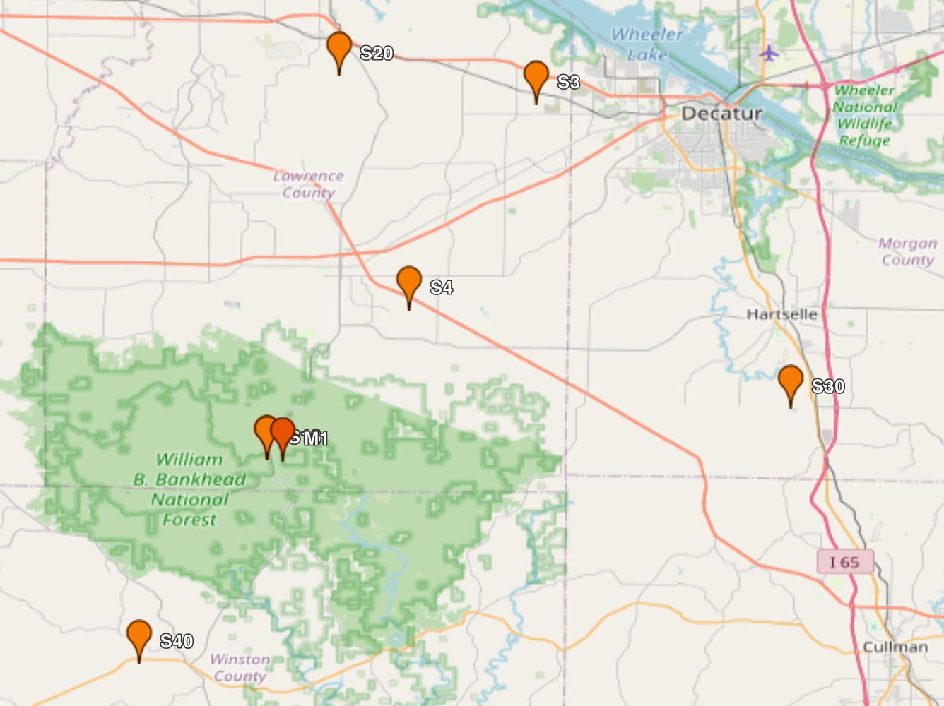
Sites
from IPython.display import HTML

HTML("""
<div style="display: flex; justify-content: center; align-items: flex-start; gap: 20px;">
    <div style="text-align: center;">
        <img src="S20.png" width="300"><br>
        <span style="font-size:18px;">S20</span>
    </div>
    <div style="text-align: center;">
        <img src="S30.png" width="300"><br>
        <span style="font-size:18px;">S30</span>
    </div>
    <div style="text-align: center;">
        <img src="S40.png" width="300"><br>
        <span style="font-size:18px;">S40</span>
    </div>
</div>
""")
Loading...
# WRF
Deciduous Broadleaf Forest
Grasslands
Croplands
Cropland/Natural Vegetation Mosaic
HTML("""
<video width="400" controls>
<source src="https://plot.dmf.arm.gov/PLOTS/bnf/bnfasimovie/20250404/bnfasimovieM1.a1.asimovie.20250404.mp4" type="video/mp4">
Your browser does not support the video tag.
</video>
""")Loading...
PBL Height
sonde_times = pd.to_datetime([
    '2025-04-04 11:30',
    '2025-04-04 17:30',
    '2025-04-04 23:30'])

data1 = [661.7, 1685.1, 1710.7]
data2 = [2241.8, 2201.9, 4037.9]
M1_PBL_ds=xr.open_dataset('M1_DL.nc')
S20_PBL_ds=xr.open_dataset('S20_DL.nc')
M1_ceil44=xr.open_dataset('M1_44.nc')
M1_ceil411=xr.open_dataset('M1_411.nc')
M1_PBL=M1_PBL_ds['M1_PBL']
S20_PBL=S20_PBL_ds['S20_PBL']
PBL_44=M1_ceil44['PBL_44']
PBL_411=M1_ceil411['PBL_411']
sonde_ds = xr.Dataset({
    'liu_liang': ('time', data1),
    'heffter': ('time', data2)
}, coords={'time': sonde_times})
Doppler Lidar: PBL defined as height where backscatter decreases the fastest.
## Apr 4
# Set paths to model outputs
path_head = '/data/project/ARM_Summer_School_2025/model/wrf/'
case_days = ['2025040406/'] #15min; 10min
for case_day in case_days:
    ds_wrf = xr.open_mfdataset(os.path.join(path_head+case_day+'run/wrfout_d01*'),concat_dim='Time',combine='nested')
    # ds_wrf
    # Create a dictionary for our ARM sites so we can easily find them in the model
    # Pull static lat/lon at first time step
    lat2d = ds_wrf['XLAT'].isel(Time=0)
    lon2d = ds_wrf['XLONG'].isel(Time=0)
    # Flatten and build KDTree
    flat_coords = np.column_stack((lat2d.values.ravel(), lon2d.values.ravel()))
    tree = cKDTree(flat_coords)
    # ARM site locations
    target_lat = [34.3425, 34.6538, 34.3848, 34.1788]
    target_lon = [-87.3382, -87.2927, -86.9279, -87.4539]
    target_coords = np.column_stack((target_lat, target_lon))
    # Find nearest indices
    _, flat_idx = tree.query(target_coords)
    i_indices, j_indices = np.unravel_index(flat_idx, lat2d.shape)
    # Create dict of site names to datasets
    site_names = ['M1', 'S20', 'S30', 'S40']
    site_datasets = {}
    for name, i, j in zip(site_names, i_indices, j_indices):
        site_datasets[name] = ds_wrf.isel(south_north=i, west_east=j).expand_dims(site=[name])
    # Subset the original WRF dataset so that it includes information for just our sites
    ds_wrf_bnf_site = xr.concat(site_datasets.values(), dim='site')
    ds_wrf_bnf_site

    var1 = ds_wrf_bnf_site['PBLH']
    var1a = ds_wrf_bnf_site['HFX'] # surface sensible heat flux
    var1b = ds_wrf_bnf_site['LH'] # surface latent heat flux
    var1c = ds_wrf_bnf_site['LWP'] # liquid water path
    LU_INDEX  = ds_wrf_bnf_site['LU_INDEX']
    VEGFRA = ds_wrf_bnf_site['VEGFRA']
    PCT_PFT = ds_wrf_bnf_site['PCT_PFT']
    LAI = ds_wrf_bnf_site['LAI']
    EMISS = ds_wrf_bnf_site['EMISS']
    ALBEDO = ds_wrf_bnf_site['ALBEDO']
    SMOIS = ds_wrf_bnf_site['SMOIS']
    RAINC = ds_wrf_bnf_site['RAINC']
    RAINNC = ds_wrf_bnf_site['RAINNC']
    xtime = pd.to_datetime(var1['XTIME'].values) - pd.Timedelta(hours=5)

    # Make the plot
    plt.figure(figsize=(10, 6),dpi=300)
    cols = ['k','gray','b','lightskyblue']
    ######################## Subplot 1 ########################
    # Sensible and latent heat fluxes
    count = 0
    for site in ['M1', 'S20']:
        plt.plot(xtime, var1.sel(site=site), c=cols[count], marker='o', linestyle='none',label=site+'_WRF')
        count+=1
    plt.plot(sonde_ds['time'], sonde_ds['liu_liang'], c='r', marker='o', linestyle='none',label='Sonde_Liu_Liang')
    plt.plot(sonde_ds['time'], sonde_ds['heffter'], c='green', marker='o', linestyle='none',label='Sonde_Heffter')
    plt.plot(M1_PBL['time'][1:-1:500],M1_PBL.values[1:-1:500],c='blue',marker='o',linestyle='none',label='DL M1')
    plt.plot(S20_PBL['time'][1:-1:500],S20_PBL.values[1:-1:500],c='orange',marker='o',linestyle='none',label='DL S20')
    plt.plot(PBL_44['time'],PBL_44.values,c='purple',marker='o',linestyle='none',label='Ceil M1')
    plt.xticks(rotation=30)
    plt.xlabel("Local Time")
    plt.ylabel("PBL Height [m]")
    plt.title("Modeled PBL Height")
    plt.legend(ncol=2)
    plt.grid(True)
    #plt.gca().xaxis.set_major_formatter(mdates.DateFormatter('%H'))
    plt.gca().xaxis.set_major_locator(mdates.HourLocator(interval=2))
    #plt.gcf().autofmt_xdate() # clean up labels
    plt.tight_layout()
    plt.show()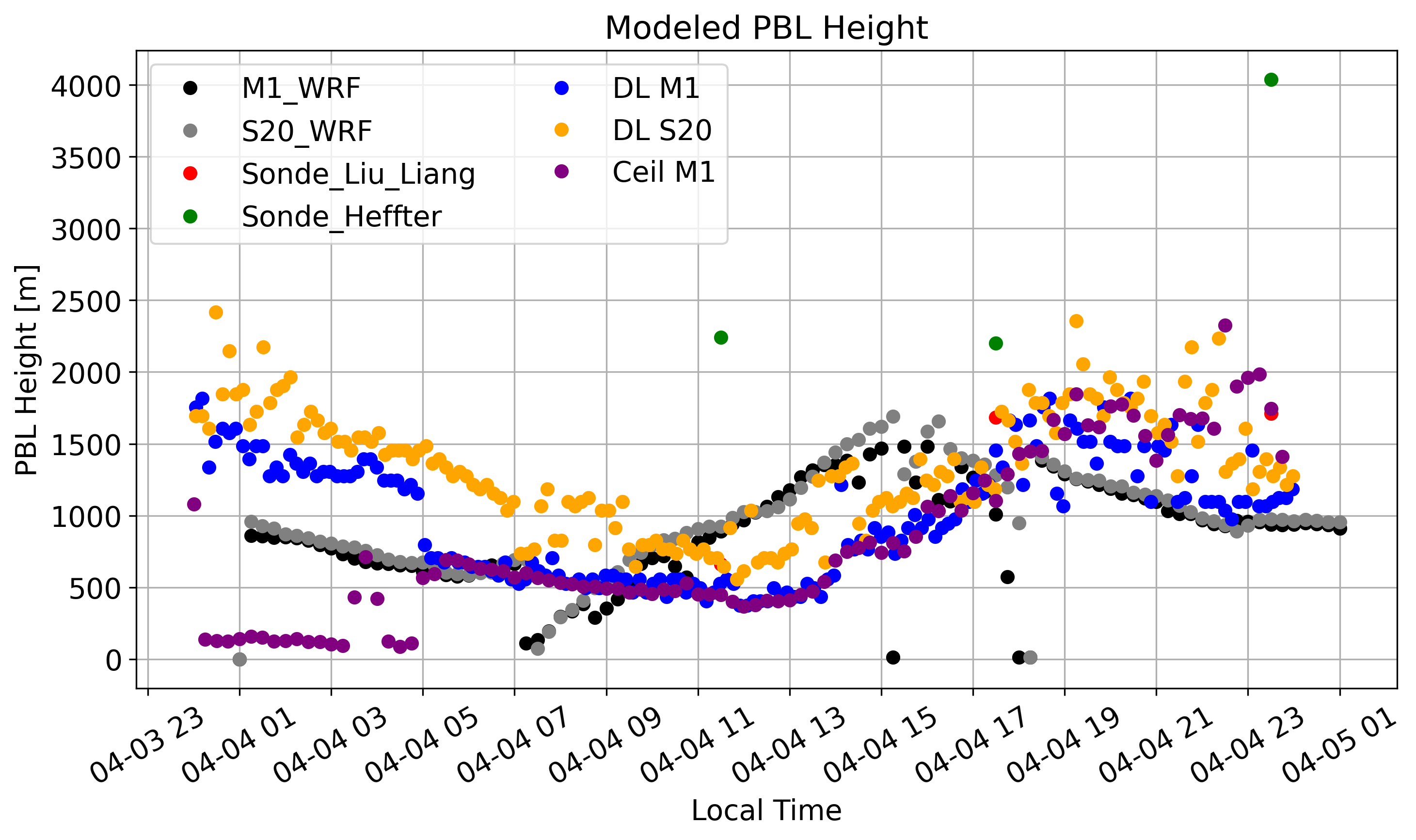
HTML("""
<video width="400" controls>
  <source src="https://plot.dmf.arm.gov/PLOTS/bnf/bnfasimovie/20250411/bnfasimovieM1.a1.asimovie.20250411.mp4" type="video/mp4">
  Your browser does not support the video tag.
</video>
""")
Loading...
sonde_times = pd.to_datetime([
    '2025-04-11 05:30',
    '2025-04-11 11:30',
    '2025-04-11 17:30',
    '2025-04-11 23:30'])

data1 = [742.69995117,516.20001221,3568,466.4]
data2 = [306.1, 306.1,3568,379.2]

sonde_ds = xr.Dataset({
    'liu_liang': ('time', data1),
    'heffter': ('time', data2)
}, coords={'time': sonde_times})
## Apr 4
# Set paths to model outputs
path_head = '/data/project/ARM_Summer_School_2025/model/wrf/'
case_days = ['2025041106/'] #15min; 10min
for case_day in case_days:
ds_wrf = xr.open_mfdataset(os.path.join(path_head+case_day+'run/wrfout_d01*'),concat_dim='Time',combine='nested')
# ds_wrf
# Create a dictionary for our ARM sites so we can easily find them in the model
# Pull static lat/lon at first time step
lat2d = ds_wrf['XLAT'].isel(Time=0)
lon2d = ds_wrf['XLONG'].isel(Time=0)
# Flatten and build KDTree
flat_coords = np.column_stack((lat2d.values.ravel(), lon2d.values.ravel()))
tree = cKDTree(flat_coords)
# ARM site locations
target_lat = [34.3425, 34.6538, 34.3848, 34.1788]
target_lon = [-87.3382, -87.2927, -86.9279, -87.4539]
target_coords = np.column_stack((target_lat, target_lon))
# Find nearest indices
_, flat_idx = tree.query(target_coords)
i_indices, j_indices = np.unravel_index(flat_idx, lat2d.shape)
# Create dict of site names to datasets
site_names = ['M1', 'S20', 'S30', 'S40']
site_datasets = {}
for name, i, j in zip(site_names, i_indices, j_indices):
site_datasets[name] = ds_wrf.isel(south_north=i, west_east=j).expand_dims(site=[name])
# Subset the original WRF dataset so that it includes information for just our sites
ds_wrf_bnf_site = xr.concat(site_datasets.values(), dim='site')
ds_wrf_bnf_site
var1 = ds_wrf_bnf_site['PBLH']
var1a = ds_wrf_bnf_site['HFX'] # surface sensible heat flux
var1b = ds_wrf_bnf_site['LH'] # surface latent heat flux
var1c = ds_wrf_bnf_site['LWP'] # liquid water path
LU_INDEX = ds_wrf_bnf_site['LU_INDEX']
VEGFRA = ds_wrf_bnf_site['VEGFRA']
PCT_PFT = ds_wrf_bnf_site['PCT_PFT']
LAI = ds_wrf_bnf_site['LAI']
EMISS = ds_wrf_bnf_site['EMISS']
ALBEDO = ds_wrf_bnf_site['ALBEDO']
SMOIS = ds_wrf_bnf_site['SMOIS']
RAINC = ds_wrf_bnf_site['RAINC']
RAINNC = ds_wrf_bnf_site['RAINNC']
xtime = pd.to_datetime(var1['XTIME'].values) - pd.Timedelta(hours=5)
# Make the plot
plt.figure(figsize=(10, 6),dpi=300)
cols = ['k','gray','b','lightskyblue']
######################## Subplot 1 ########################
# Sensible and latent heat fluxes
count = 0
for site in ['M1', 'S20']:
plt.plot(xtime, var1.sel(site=site), c=cols[count], marker='o', linestyle='none',label=site+'_WRF')
count+=1
plt.plot(sonde_ds['time'], sonde_ds['liu_liang'], c='r', marker='o', linestyle='none',label='Sonde_Liu_Liang')
plt.plot(sonde_ds['time'], sonde_ds['heffter'], c='green', marker='o', linestyle='none',label='Sonde_Heffter')
plt.plot(PBL_411['time'],PBL_411.values,c='purple',marker='o',linestyle='none',label='Ceil M1')
plt.xticks(rotation=30)
plt.xlabel("Local Time")
plt.ylabel("PBL Height [m]")
plt.title("Modeled PBL Height")
plt.legend()
plt.grid(True)
#plt.gca().xaxis.set_major_formatter(mdates.DateFormatter('%H'))
plt.gca().xaxis.set_major_locator(mdates.HourLocator(interval=2))
#plt.gcf().autofmt_xdate() # clean up labels
plt.tight_layout()
plt.show()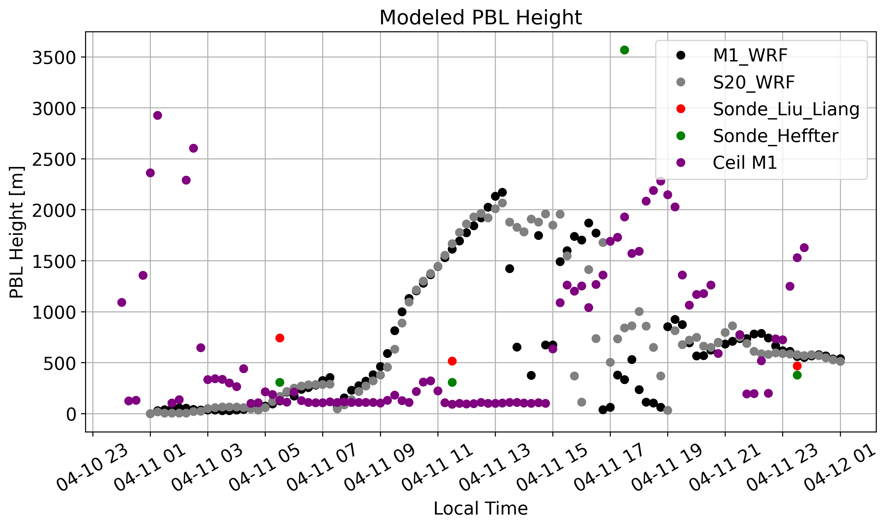
WRF
M1  – Deciduous Broadleaf Forest
S20 – Grasslands
S30 – Croplands
S40 – Cropland/Natural Vegetation Mosaic
# Set paths to model outputs
path_head = '/data/project/ARM_Summer_School_2025/model/wrf/'
case_days = ['2025040406/'] #15min; 10min
for case_day in case_days:
ds_wrf = xr.open_mfdataset(os.path.join(path_head+case_day+'run/wrfout_d01*'),concat_dim='Time',combine='nested')
# ds_wrf
# Create a dictionary for our ARM sites so we can easily find them in the model
# Pull static lat/lon at first time step
lat2d = ds_wrf['XLAT'].isel(Time=0)
lon2d = ds_wrf['XLONG'].isel(Time=0)
# Flatten and build KDTree
flat_coords = np.column_stack((lat2d.values.ravel(), lon2d.values.ravel()))
tree = cKDTree(flat_coords)
# ARM site locations
target_lat = [34.3425, 34.6538, 34.3848, 34.1788]
target_lon = [-87.3382, -87.2927, -86.9279, -87.4539]
target_coords = np.column_stack((target_lat, target_lon))
# Find nearest indices
_, flat_idx = tree.query(target_coords)
i_indices, j_indices = np.unravel_index(flat_idx, lat2d.shape)
# Create dict of site names to datasets
site_names = ['M1', 'S20', 'S30', 'S40']
site_datasets = {}
for name, i, j in zip(site_names, i_indices, j_indices):
site_datasets[name] = ds_wrf.isel(south_north=i, west_east=j).expand_dims(site=[name])
# Subset the original WRF dataset so that it includes information for just our sites
ds_wrf_bnf_site = xr.concat(site_datasets.values(), dim='site')
ds_wrf_bnf_site
var1 = ds_wrf_bnf_site['PBLH']
var1a = ds_wrf_bnf_site['HFX'] # surface sensible heat flux
var1b = ds_wrf_bnf_site['LH'] # surface latent heat flux
var1c = ds_wrf_bnf_site['LWP'] # liquid water path
LU_INDEX = ds_wrf_bnf_site['LU_INDEX']
VEGFRA = ds_wrf_bnf_site['VEGFRA']
PCT_PFT = ds_wrf_bnf_site['PCT_PFT']
LAI = ds_wrf_bnf_site['LAI']
EMISS = ds_wrf_bnf_site['EMISS']
ALBEDO = ds_wrf_bnf_site['ALBEDO']
SMOIS = ds_wrf_bnf_site['SMOIS']
RAINC = ds_wrf_bnf_site['RAINC']
RAINNC = ds_wrf_bnf_site['RAINNC']
xtime = pd.to_datetime(var1['XTIME'].values) - pd.Timedelta(hours=5)
# Make the plot
plt.figure(figsize=(16, 13),dpi=300)
cols = ['k','gray','b','lightskyblue']
######################## Subplot 1 ########################
# Sensible and latent heat fluxes
plt.subplot(2,2,1)
count = 0
for site in var1.site.values:
plt.plot(xtime, var1.sel(site=site), c=cols[count], label=site)
count+=1
plt.xticks(rotation=30)
plt.xlabel("Time")
plt.ylabel("PBL Height [m]")
plt.title("Modeled PBL Height")
plt.legend()
plt.grid(True)
#plt.gca().xaxis.set_major_formatter(mdates.DateFormatter('%H'))
#plt.gca().xaxis.set_major_locator(mdates.HourLocator(interval=2))
######################## Subplot 2 ########################
plt.subplot(2,2,2)
count = 0
for site in var1a.site.values:
plt.plot(xtime, var1a.sel(site=site), c=cols[count], label=site)
plt.plot(xtime, var1b.sel(site=site), c=cols[count], ls='--')
count+=1
plt.xticks(rotation=30)
plt.xlabel("Time")
plt.ylabel("Heat Fluxes [W m$^{-2}$]")
plt.title("Modeled Surface Sensible (solid) and\nLatent (dashed) Heat Fluxes")
plt.legend()
plt.grid(True)
######################## Subplot 3 ########################
# Sensible and latent heat fluxes
plt.subplot(2,2,3)
count = 0
for site in var1.site.values:
plt.plot(xtime, SMOIS.sel(site=site)[:,0], c=cols[count], label=site)
count+=1
plt.xticks(rotation=30)
plt.xlabel("Time")
plt.ylabel("Soil Moisture [$m^3 m^{-3}$]")
plt.title("Modeled Soil Moisture")
plt.legend()
plt.grid(True)
# Liquid water path
plt.subplot(2,2,4)
count = 0
for site in var1.site.values:
#plt.plot(var2['XTIME'], var2.sel(site=site), c=cols[count], label=site)
plt.plot(xtime, RAINNC.sel(site=site), c=cols[count], label=site)
count+=1
plt.xticks(rotation=30)
plt.xlabel("Time")
#plt.ylabel("Liquid Water Path [kg m$^{-2}$]")
#plt.title("Modeled Liquid Water Path (solid) at ARM Sites")
plt.ylabel("Precipitation [mm]")
plt.title("Modeled Non-convective Precipitation")
plt.legend()
plt.grid(True)
#plt.gcf().autofmt_xdate() # clean up labels
plt.tight_layout()
plt.show()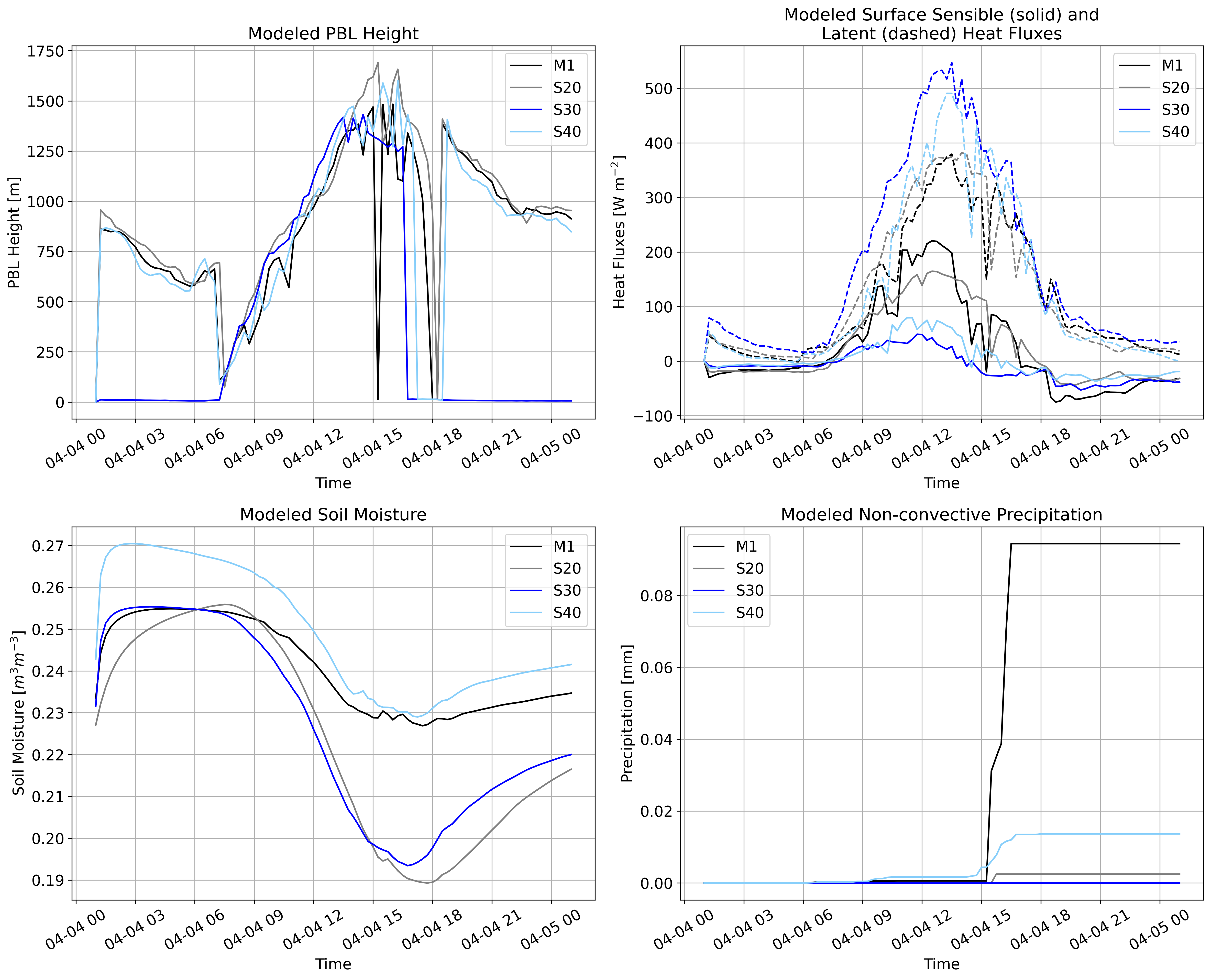
# Set paths to model outputs
path_head = '/data/project/ARM_Summer_School_2025/model/wrf/'
case_days = ['2025041106/'] #15min; 10min
for case_day in case_days:
    ds_wrf = xr.open_mfdataset(os.path.join(path_head+case_day+'run/wrfout_d01*'),concat_dim='Time',combine='nested')
    # ds_wrf
    # Create a dictionary for our ARM sites so we can easily find them in the model
    # Pull static lat/lon at first time step
    lat2d = ds_wrf['XLAT'].isel(Time=0)
    lon2d = ds_wrf['XLONG'].isel(Time=0)
    # Flatten and build KDTree
    flat_coords = np.column_stack((lat2d.values.ravel(), lon2d.values.ravel()))
    tree = cKDTree(flat_coords)
    # ARM site locations
    target_lat = [34.3425, 34.6538, 34.3848, 34.1788]
    target_lon = [-87.3382, -87.2927, -86.9279, -87.4539]
    target_coords = np.column_stack((target_lat, target_lon))
    # Find nearest indices
    _, flat_idx = tree.query(target_coords)
    i_indices, j_indices = np.unravel_index(flat_idx, lat2d.shape)
    # Create dict of site names to datasets
    site_names = ['M1', 'S20', 'S30', 'S40']
    site_datasets = {}
    for name, i, j in zip(site_names, i_indices, j_indices):
        site_datasets[name] = ds_wrf.isel(south_north=i, west_east=j).expand_dims(site=[name])
    # Subset the original WRF dataset so that it includes information for just our sites
    ds_wrf_bnf_site = xr.concat(site_datasets.values(), dim='site')
    ds_wrf_bnf_site

    var1 = ds_wrf_bnf_site['PBLH']
    var1a = ds_wrf_bnf_site['HFX'] # surface sensible heat flux
    var1b = ds_wrf_bnf_site['LH'] # surface latent heat flux
    var1c = ds_wrf_bnf_site['LWP'] # liquid water path
    LU_INDEX  = ds_wrf_bnf_site['LU_INDEX']
    VEGFRA = ds_wrf_bnf_site['VEGFRA']
    PCT_PFT = ds_wrf_bnf_site['PCT_PFT']
    LAI = ds_wrf_bnf_site['LAI']
    EMISS = ds_wrf_bnf_site['EMISS']
    ALBEDO = ds_wrf_bnf_site['ALBEDO']
    SMOIS = ds_wrf_bnf_site['SMOIS']
    RAINC = ds_wrf_bnf_site['RAINC']
    RAINNC = ds_wrf_bnf_site['RAINNC']
    xtime = pd.to_datetime(var1['XTIME'].values) - pd.Timedelta(hours=5)

    # Make the plot
    plt.figure(figsize=(16, 13),dpi=300)
    cols = ['k','gray','b','lightskyblue']
    ######################## Subplot 1 ########################
    # Sensible and latent heat fluxes
    plt.subplot(2,2,1)
    count = 0
    for site in var1.site.values:
        plt.plot(xtime, var1.sel(site=site), c=cols[count], label=site)
        count+=1
    plt.xticks(rotation=30)
    plt.xlabel("Time")
    plt.ylabel("PBL Height [m]")
    plt.title("Modeled PBL Height")
    plt.legend()
    plt.grid(True)
    #plt.gca().xaxis.set_major_formatter(mdates.DateFormatter('%H'))
    #plt.gca().xaxis.set_major_locator(mdates.HourLocator(interval=2))
    ######################## Subplot 2 ########################
    plt.subplot(2,2,2)
    count = 0
    for site in var1a.site.values:
        plt.plot(xtime, var1a.sel(site=site), c=cols[count], label=site)
        plt.plot(xtime, var1b.sel(site=site), c=cols[count], ls='--')
        count+=1
    plt.xticks(rotation=30)
    plt.xlabel("Time")
    plt.ylabel("Heat Fluxes [W m$^{-2}$]")
    plt.title("Modeled Surface Sensible (solid) and\nLatent (dashed) Heat Fluxes")
    plt.legend()
    plt.grid(True)
    ######################## Subplot 3 ########################
    # Sensible and latent heat fluxes
    plt.subplot(2,2,3)
    count = 0
    for site in var1.site.values:
        plt.plot(xtime, SMOIS.sel(site=site)[:,0], c=cols[count], label=site)
        count+=1
    plt.xticks(rotation=30)
    plt.xlabel("Time")
    plt.ylabel("Soil Moisture [$m^3 m^{-3}$]")
    plt.title("Modeled Soil Moisture")
    plt.legend()
    plt.grid(True)

    # Liquid water path
    plt.subplot(2,2,4)
    count = 0
    for site in var1.site.values:
        #plt.plot(var2['XTIME'], var2.sel(site=site), c=cols[count], label=site)
        plt.plot(xtime, RAINNC.sel(site=site), c=cols[count], label=site)
        count+=1
    plt.xticks(rotation=30)
    plt.xlabel("Time")
    #plt.ylabel("Liquid Water Path [kg m$^{-2}$]")
    #plt.title("Modeled Liquid Water Path (solid) at ARM Sites")
    plt.ylabel("Precipitation [mm]")
    plt.title("Modeled Non-convective Precipitation")
    plt.legend()
    plt.grid(True)
    #plt.gcf().autofmt_xdate() # clean up labels
    plt.tight_layout()
    plt.show()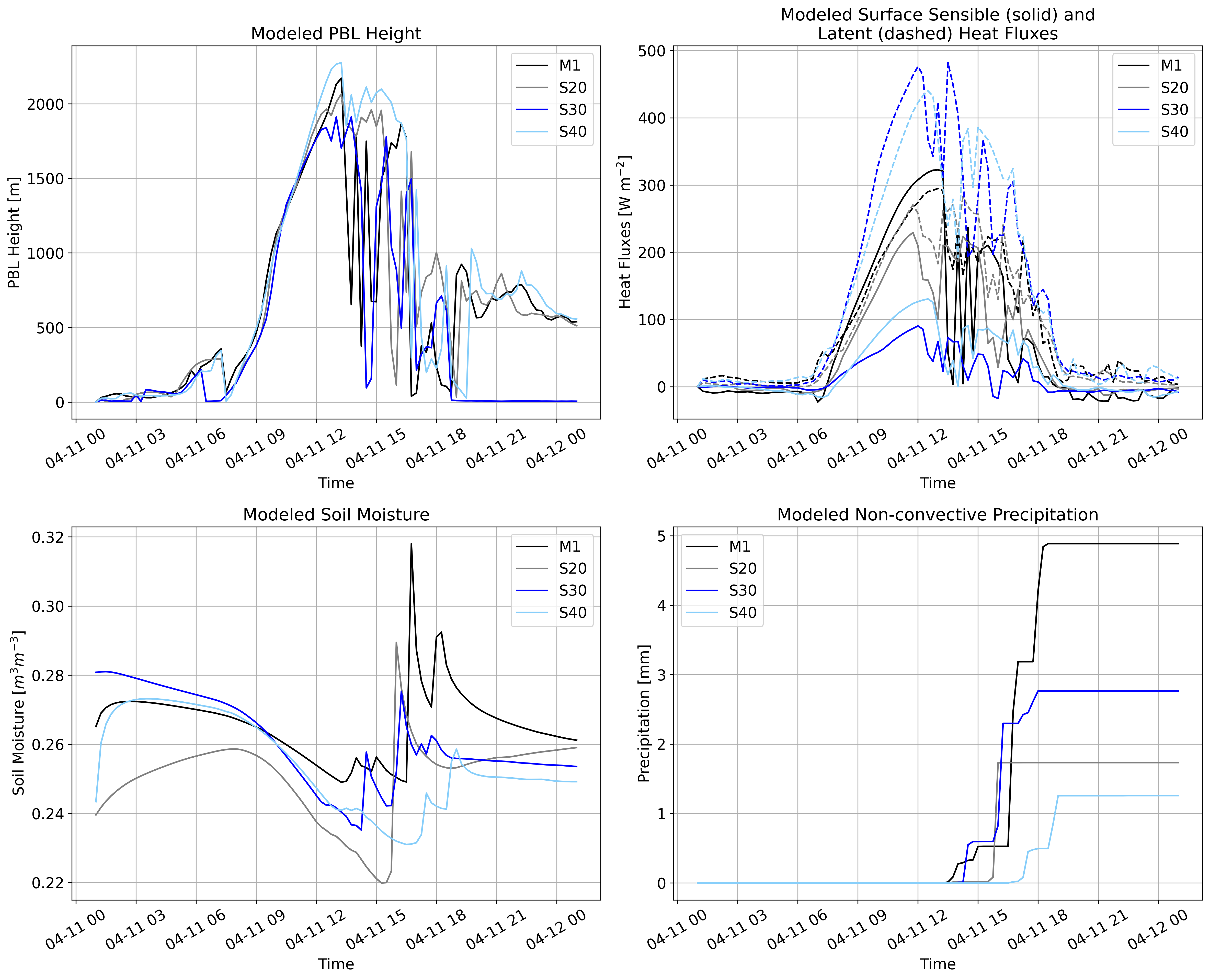
HTML("""
<div style="display: flex; justify-content: center; align-items: flex-start; gap: 20px;">
    <div style="text-align: center;">
        <img src="SHF.png" width="1000"><br>
        <span style="font-size:18px;">S20</span>
    </div>
</div>
""")
Loading...
HTML("""
<div style="display: flex; justify-content: center; align-items: flex-start; gap: 20px;">
    <div style="text-align: center;">
        <img src="download.png" width="1000"><br>
        <span style="font-size:18px;">S20</span>
    </div>
</div>
""")
Loading...