import os
import numpy as np
import xarray as xr
import matplotlib.pyplot as plt
import matplotlib.colors as colors

import getpass
import act
# Note - recommended ARM Live token to be set as an environmental variable
# Check for env variables, otherwise set your username and token here!
if "ARM_USERNAME" in os.environ:
arm_username = os.getenv("ARM_USERNAME")
else:
arm_username = input("Enter ARM username: ").strip()
if "ARM_TOKEN" in os.environ:
arm_token = os.getenv("ARM_TOKEN")
else:
arm_token = getpass.getpass("Enter ARM token (hidden): ").strip()
# Set the datastream and start/enddates
mw1 = 'nsamwrlosC1.b1' ## mwrlos
mw2 = "nsamwrret1liljclouC1.c2" ## MWRRET1LILJCLOU
mw3 = "nsamwrhfC1.b1" #"MWRHF"
weather_data = "nsametC1.b1"
cloud_phase = "nsathermocldphaseC1"
startdate = '2015-06-10'
enddate = '2015-06-20'
# Use ACT to easily download the data. Watch for the data citation! Show some support
# for ARM's instrument experts and cite their data if you use it in a publication
result_mr1 = act.discovery.download_arm_data(arm_username, arm_token, mw1, startdate, enddate)
print('1')
result_mr2 = act.discovery.download_arm_data(arm_username, arm_token, mw2, startdate, enddate)
print('2')
result_mr3 = act.discovery.download_arm_data(arm_username, arm_token, mw3, startdate, enddate)
print('3')
wd_1 = act.discovery.download_arm_data(arm_username, arm_token, weather_data, startdate, enddate)
print('1')
cloud_phase_1 = act.discovery.download_arm_data(arm_username, arm_token, cloud_phase, startdate, enddate)
print('cloud_phase')Enter ARM username: ssingh45
Enter ARM token (hidden): ········
[DOWNLOADING] nsamwrlosC1.b1.20150610.000040.cdf
[DOWNLOADING] nsamwrlosC1.b1.20150611.000000.cdf
[DOWNLOADING] nsamwrlosC1.b1.20150612.000011.cdf
[DOWNLOADING] nsamwrlosC1.b1.20150613.000005.cdf
[DOWNLOADING] nsamwrlosC1.b1.20150614.000000.cdf
[DOWNLOADING] nsamwrlosC1.b1.20150615.000000.cdf
[DOWNLOADING] nsamwrlosC1.b1.20150616.000000.cdf
[DOWNLOADING] nsamwrlosC1.b1.20150617.000017.cdf
[DOWNLOADING] nsamwrlosC1.b1.20150618.000032.cdf
[DOWNLOADING] nsamwrlosC1.b1.20150619.000020.cdf
[DOWNLOADING] nsamwrlosC1.b1.20150620.000000.cdf

If you use these data to prepare a publication, please cite:

Cadeddu, M. Microwave Radiometer (MWRLOS), 2015-06-10 to 2015-06-20, North Slope
Alaska (NSA), Central Facility, Barrow AK (C1). Atmospheric Radiation
Measurement (ARM) User Facility. https://doi.org/10.5439/1999490

1
[DOWNLOADING] nsamwrret1liljclouC1.c2.20150610.000040.nc
[DOWNLOADING] nsamwrret1liljclouC1.c2.20150611.000000.nc
[DOWNLOADING] nsamwrret1liljclouC1.c2.20150612.000011.nc
[DOWNLOADING] nsamwrret1liljclouC1.c2.20150613.000005.nc
[DOWNLOADING] nsamwrret1liljclouC1.c2.20150614.000000.nc
[DOWNLOADING] nsamwrret1liljclouC1.c2.20150615.000000.nc
[DOWNLOADING] nsamwrret1liljclouC1.c2.20150616.000000.nc
[DOWNLOADING] nsamwrret1liljclouC1.c2.20150617.000017.nc
[DOWNLOADING] nsamwrret1liljclouC1.c2.20150618.000032.nc
[DOWNLOADING] nsamwrret1liljclouC1.c2.20150619.000020.nc
[DOWNLOADING] nsamwrret1liljclouC1.c2.20150620.000000.nc

If you use these data to prepare a publication, please cite:

Zhang, D. MWR Retrievals (MWRRET1LILJCLOU), 2015-06-10 to 2015-06-20, North
Slope Alaska (NSA), Central Facility, Barrow AK (C1). Atmospheric Radiation
Measurement (ARM) User Facility. https://doi.org/10.5439/1027369

2
No files returned or url status error.
Check datastream name, start, and end date.
3
[DOWNLOADING] nsametC1.b1.20150610.000000.cdf
[DOWNLOADING] nsametC1.b1.20150611.000000.cdf
[DOWNLOADING] nsametC1.b1.20150612.000000.cdf
[DOWNLOADING] nsametC1.b1.20150612.180000.cdf
[DOWNLOADING] nsametC1.b1.20150613.000000.cdf
[DOWNLOADING] nsametC1.b1.20150614.000000.cdf
[DOWNLOADING] nsametC1.b1.20150615.000000.cdf
[DOWNLOADING] nsametC1.b1.20150616.000000.cdf
[DOWNLOADING] nsametC1.b1.20150617.000000.cdf
[DOWNLOADING] nsametC1.b1.20150618.000000.cdf
[DOWNLOADING] nsametC1.b1.20150619.000000.cdf
[DOWNLOADING] nsametC1.b1.20150620.000000.cdf

If you use these data to prepare a publication, please cite:

Kyrouac, J., Shi, Y., & Tuftedal, M. Surface Meteorological Instrumentation
(MET), 2015-06-10 to 2015-06-20, North Slope Alaska (NSA), Central Facility,
Barrow AK (C1). Atmospheric Radiation Measurement (ARM) User Facility.
https://doi.org/10.5439/1786358

1
[DOWNLOADING] nsathermocldphaseC1.c0.20150610.000000.nc
[DOWNLOADING] nsathermocldphaseC1.c0.20150611.000000.nc
[DOWNLOADING] nsathermocldphaseC1.c0.20150612.000000.nc
[DOWNLOADING] nsathermocldphaseC1.c0.20150613.000000.nc
[DOWNLOADING] nsathermocldphaseC1.c0.20150614.000000.nc
[DOWNLOADING] nsathermocldphaseC1.c0.20150615.000000.nc
[DOWNLOADING] nsathermocldphaseC1.c0.20150616.000000.nc
[DOWNLOADING] nsathermocldphaseC1.c0.20150617.000000.nc
[DOWNLOADING] nsathermocldphaseC1.c0.20150618.000000.nc
[DOWNLOADING] nsathermocldphaseC1.c0.20150619.000000.nc
[DOWNLOADING] nsathermocldphaseC1.c0.20150620.000000.nc

If you use these data to prepare a publication, please cite:

Please check your arguments. No DOI Found

cloud_phase
ds_mr1 = act.io.read_arm_netcdf(result_mr1)
ds_mr2 = act.io.read_arm_netcdf(result_mr2)
ds_met1 = act.io.read_arm_netcdf(wd_1)
cloud_phase_1 = act.io.read_arm_netcdf(cloud_phase_1)
ERROR 1: PROJ: proj_create_from_database: Open of /opt/conda/share/proj failed
precipation
ds_met1["pwd_cumul_rain"].plot()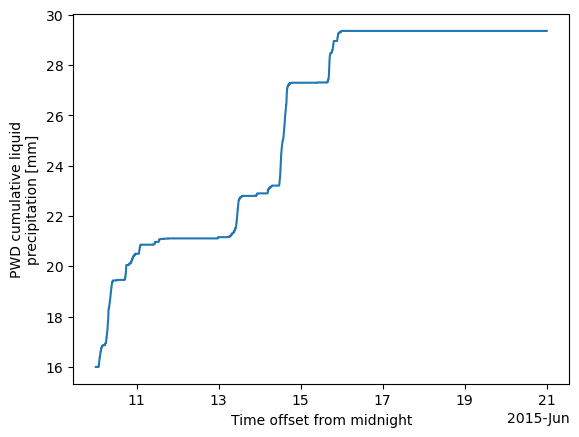
ds_met1["pwd_cumul_snow"].plot()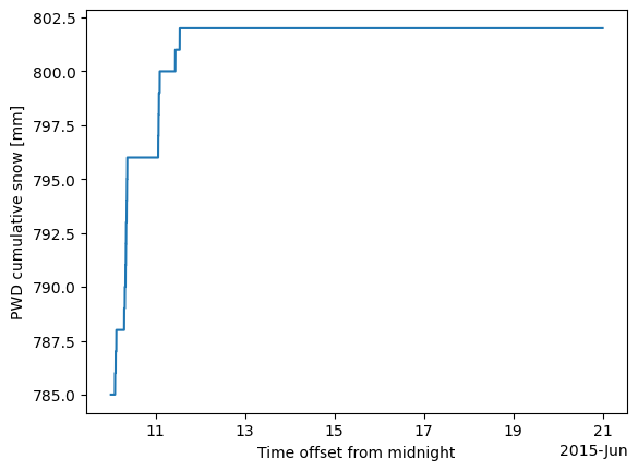
radiometer
ds_mr1
# vap, qc_vap, liq, qc_liq
Loading...
ds_mr1['vap'].plot()
ds_mr1['liq'].plot()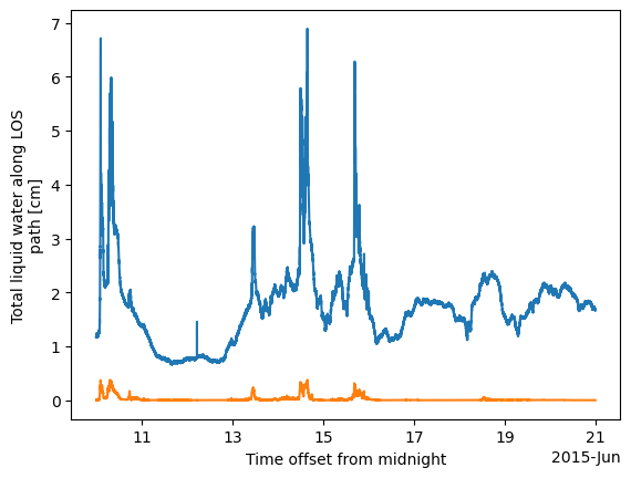
ds_mr2Loading...
# ds_mr2['cloud_base_height'].sel(time=slice('2015-06-12T00:00', '2015-06-17T00:00')).plot()ds_mr2['orig_pwv'].plot()
plt.ylim(0, 5)(0.0, 5.0)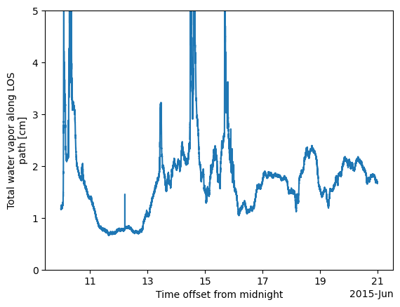
ds_mr2['orig_lwp'].plot()
# plt.ylim(0, 5)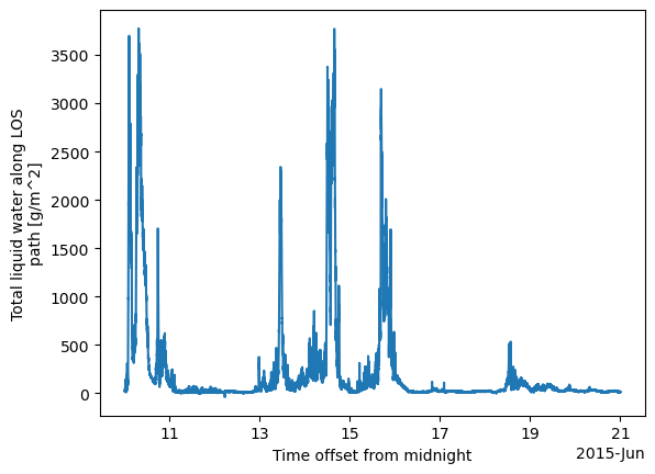
ds_mr2['orig_lwp'].plot()
# plt.ylim(0, 5)cloud_phase_1Loading...
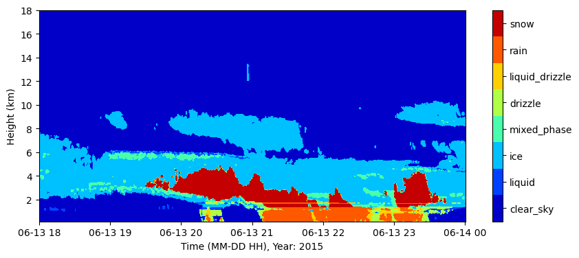
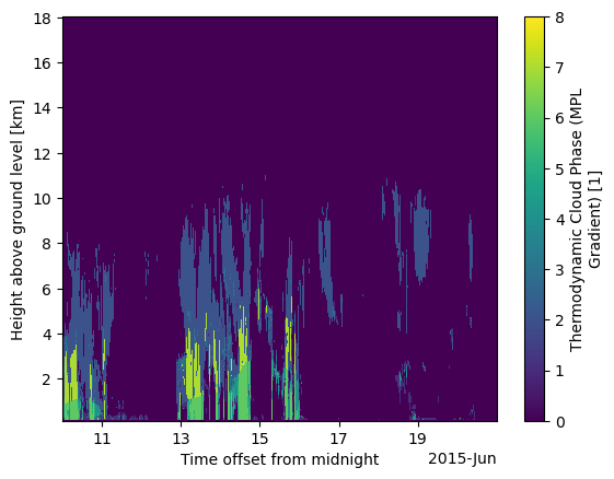
cloud_phase_1["cloud_phase_mplgr"].transpose().plot()
# flag_values :
#     [0 1 2 3 4 5 6 7 8]
# flag_meanings :
#     clear_sky liquid ice mixed_phase drizzle liquid_drizzle rain snow unknown
cloud_phase_1["cloud_phase_mplgr"][:, 40].plot()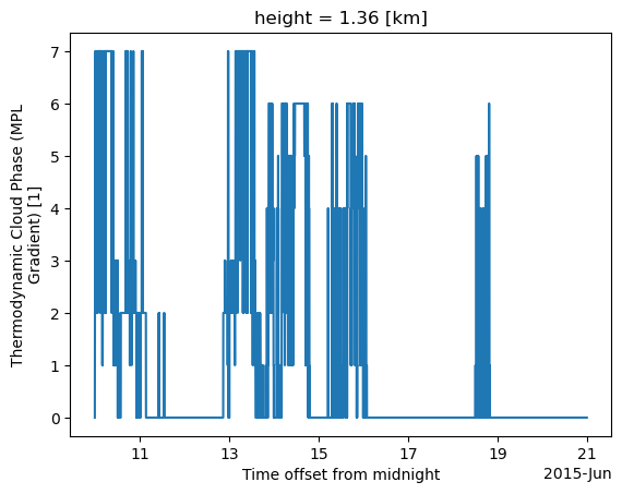
cloud_phase_1["cloud_phase_mplgr"].sel(time=slice('2015-06-13T18:00', '2015-06-14T00:00')).transpose().plot()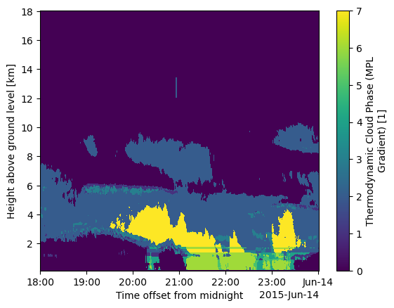
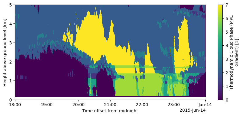
cloud_phase_1["cloud_phase_mplgr"].sel(time=slice('2015-06-13T18:00', '2015-06-14T00:00')).transpose().plot()xx = cloud_phase_1["cloud_phase_mplgr"].sel(time=slice('2015-06-13T18:00', '2015-06-14T00:00'))
threshold = 7
da_masked = xx.where(xx <= threshold, other=np.nan)
plt.figure(figsize=(10, 4))
da_masked.transpose().plot(ylim=(0, 5))
threshold = 7
da_masked = xx.where(xx <= threshold, other=np.nan)
plt.figure(figsize=(8, 4))
da_masked.transpose().plot()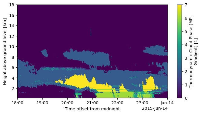
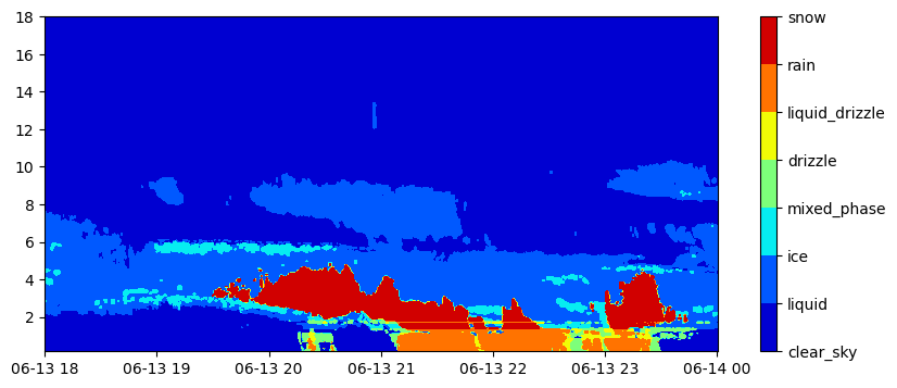
plt.figure(figsize=(10, 4))
levels = [0.0, 1.0, 2.0, 3.0, 4.0, 5.0, 6.0, 7.0]
contour_filled = plt.contourf(np.array(xx.time), np.array(xx.height), np.array(xx.transpose()), levels=levels, cmap="jet")

# 3. Create the colorbar
cbar = plt.colorbar(contour_filled)
cbar.set_ticks([0.0, 1.0, 2.0, 3.0, 4.0, 5.0, 6.0, 7.0])

# 5. Replace those tick positions with your custom text
cbar.set_ticklabels(["clear_sky", "liquid", "ice", "mixed_phase", "drizzle", "liquid_drizzle", "rain", "snow"])

plt.title('')
plt.show()
plt.figure(figsize=(10, 4))
levels = [0.0, 1.0, 2.0, 3.0, 4.0, 5.0, 6.0, 7.0, 8.0]
contour_filled = plt.contourf(np.array(xx.time), np.array(xx.height), np.array(xx.transpose())+0.5, levels=levels, cmap="jet")

# 3. Create the colorbar
cbar = plt.colorbar(contour_filled)
cbar.set_ticks(np.array([0.0, 1.0, 2.0, 3.0, 4.0, 5.0, 6.0, 7.0])+0.5)

# 5. Replace those tick positions with your custom text
cbar.set_ticklabels(["clear_sky", "liquid", "ice", "mixed_phase", "drizzle", "liquid_drizzle", "rain", "snow"])

plt.title('')
plt.xlabel('Time (MM-DD HH), Year: 2015')
plt.ylabel('Height (km)')
plt.ylim()
plt.show()