import act
import numpy as np
import xarray as xr
import matplotlib.pyplot as plt
from scipy.stats import linregress
import matplotlib.colors as colors
import pandas as pd
import matplotlib.dates as mdates
# Set your username and token here!
username = 'sanielson'
token = '467abc05f4c61fde'
startdate = '2025-02-07'
enddate = '2025-04-30T23:59:59'
# Set the datastream and start/enddates
datastream_sebs_s40 = 'bnfsebsS40.b1'
datastream_sebs_s30 = 'bnfsebsS30.b1'
datastream_sebs_s20 = 'bnfsebsS20.b1'
# Use ACT to easily download the data. Watch for the data citation! Show some support
# for ARM's instrument experts and cite their data if you use it in a publication
result_sebs_s40 = act.discovery.download_arm_data(username, token, datastream_sebs_s40, startdate, enddate)
result_sebs_s30 = act.discovery.download_arm_data(username, token, datastream_sebs_s30, startdate, enddate)
result_sebs_s20 = act.discovery.download_arm_data(username, token, datastream_sebs_s20, startdate, enddate)
datastream_ecor_s40 = 'bnfecorsfS40.b1'
datastream_ecor_s30 = 'bnfecorsfS30.b1'
datastream_ecor_s20 = 'bnfecorsfS20.b1'
result_ecor_s40 = act.discovery.download_arm_data(username, token, datastream_ecor_s40, startdate, enddate)
result_ecor_s30 = act.discovery.download_arm_data(username, token, datastream_ecor_s30, startdate, enddate)
result_ecor_s20 = act.discovery.download_arm_data(username, token, datastream_ecor_s20, startdate, enddate)
datastream_sirs_s40 = 'bnfsirsS40.b1'
datastream_sirs_s30 = 'bnfsirsS30.b1'
datastream_sirs_s20 = 'bnfsirsS20.b1'
result_sirs_s40 = act.discovery.download_arm_data(username, token, datastream_sirs_s40, startdate, enddate)
result_sirs_s30 = act.discovery.download_arm_data(username, token, datastream_sirs_s30, startdate, enddate)
result_sirs_s20 = act.discovery.download_arm_data(username, token, datastream_sirs_s20, startdate, enddate)Fetching long content....
# Let's read in the data using ACT and check out the data
ds_sebs_s40 = act.io.read_arm_netcdf(result_sebs_s40)
ds_sebs_s30 = act.io.read_arm_netcdf(result_sebs_s30)
ds_sebs_s20 = act.io.read_arm_netcdf(result_sebs_s20)

ds_sebs_s40
ds_sebs_s30
ds_sebs_s20
ERROR 1: PROJ: proj_create_from_database: Open of /opt/conda/share/proj failed
Loading...
#ECOR has sensible and latent heat flux together
ds_ecor_s40 = act.io.read_arm_netcdf(result_ecor_s40)
ds_ecor_s30 = act.io.read_arm_netcdf(result_ecor_s30)
ds_ecor_s20 = act.io.read_arm_netcdf(result_ecor_s20)

ds_ecor_s40
ds_ecor_s30
ds_ecor_s20
Loading...
# Let's read in the data using ACT and check out the data
ds_sirs_s40 = act.io.read_arm_netcdf(result_sirs_s40)
ds_sirs_s30 = act.io.read_arm_netcdf(result_sirs_s30)
ds_sirs_s20 = act.io.read_arm_netcdf(result_sirs_s20)

ds_sirs_s40
ds_sirs_s30
ds_sirs_s20
Loading...
ds_sirs_s40.clean.cleanup()
ds_sirs_s30.clean.cleanup()
ds_sirs_s20.clean.cleanup()
net_radiation_s40 = (ds_sirs_s40['down_long_hemisp1'] - ds_sirs_s40['up_long_hemisp']) + (ds_sirs_s40['down_short_hemisp'] - ds_sirs_s40['up_short_hemisp'])
net_radiation_s30 = (ds_sirs_s30['down_long_hemisp1'] - ds_sirs_s30['up_long_hemisp']) + (ds_sirs_s30['down_short_hemisp'] - ds_sirs_s30['up_short_hemisp'])
net_radiation_s20 = (ds_sirs_s20['down_long_hemisp1'] - ds_sirs_s20['up_long_hemisp']) + (ds_sirs_s20['down_short_hemisp'] - ds_sirs_s20['up_short_hemisp'])
#net radiation calculations
net_radiation_s40.plot()
net_radiation_s30.plot()
net_radiation_s20.plot()
plt.title('Net Radiation')
plt.ylabel('Radiation')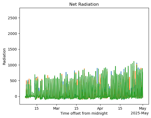
ds_sebs_s40.clean.cleanup()
ds_sebs_s30.clean.cleanup()
ds_sebs_s20.clean.cleanup()
avail_e_s40 = net_radiation_s40 - ds_sebs_s40['surface_soil_heat_flux_avg']
avail_e_s30 = net_radiation_s30 - ds_sebs_s30['surface_soil_heat_flux_avg']
avail_e_s20 = net_radiation_s20 - ds_sebs_s20['surface_soil_heat_flux_avg']#net radiation calculations
avail_e_s40.plot()
avail_e_s30.plot()
avail_e_s20.plot()
plt.title('Net Radiation')
plt.ylabel('Radiation')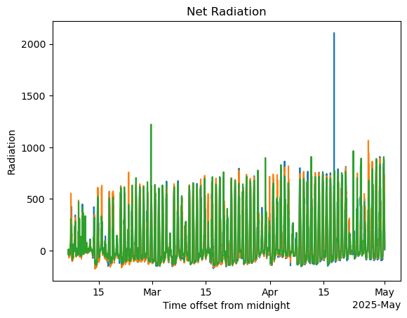
ds_ecor_s40.clean.cleanup()
ds_ecor_s30.clean.cleanup()
ds_ecor_s20.clean.cleanup()
turb_flux_s40 = ds_ecor_s40['sensible_heat_flux'] + ds_ecor_s40['latent_flux']
turb_flux_s30 = ds_ecor_s30['sensible_heat_flux'] + ds_ecor_s30['latent_flux']
turb_flux_s20 = ds_ecor_s20['sensible_heat_flux'] + ds_ecor_s20['latent_flux']#net radiation calculations
turb_flux_s40.plot()
turb_flux_s30.plot()
turb_flux_s20.plot()
plt.title('Turbulent Flux')
plt.ylabel('Radiation')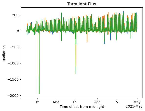
turb_flux_aligned_s40, avail_e_aligned_s40 = xr.align(turb_flux_s40, avail_e_s40, join = 'inner')
turb_flux_aligned_s30, avail_e_aligned_s30 = xr.align(turb_flux_s40, avail_e_s30, join = 'inner')
turb_flux_aligned_s20, avail_e_aligned_s20 = xr.align(turb_flux_s40, avail_e_s20, join = 'inner')
# --- Step 1: Timezone-aware time-of-day coordinate ---
def add_time_of_day(da):
utc_times = pd.to_datetime(da.time.values).tz_localize('UTC')
central_times = utc_times.tz_convert('US/Central')
rounded = central_times.floor('30min')
time_of_day_strs = xr.DataArray(rounded.strftime('%H:%M'), coords={'time': da.time}, dims='time')
return da.assign_coords(time_of_day=time_of_day_strs)
# --- Step 2: Assign to each variable ---
le_td_s40 = add_time_of_day(ds_ecor_s40['latent_flux'])
le_td_s30 = add_time_of_day(ds_ecor_s30['latent_flux'])
le_td_s20 = add_time_of_day(ds_ecor_s20['latent_flux'])
h_td_s40 = add_time_of_day(ds_ecor_s40['sensible_heat_flux'])
h_td_s30 = add_time_of_day(ds_ecor_s30['sensible_heat_flux'])
h_td_s20 = add_time_of_day(ds_ecor_s20['sensible_heat_flux'])
rn_td_s40 = add_time_of_day(net_radiation_s40)
rn_td_s30 = add_time_of_day(net_radiation_s30)
rn_td_s20 = add_time_of_day(net_radiation_s20)
g_td_s40 = add_time_of_day(ds_sebs_s40['surface_soil_heat_flux_avg'])
g_td_s30 = add_time_of_day(ds_sebs_s30['surface_soil_heat_flux_avg'])
g_td_s20 = add_time_of_day(ds_sebs_s20['surface_soil_heat_flux_avg'])
# --- Step 3: Group by time-of-day and average ---
le_avg_s40 = le_td_s40.groupby('time_of_day').mean('time')
le_avg_s30 = le_td_s30.groupby('time_of_day').mean('time')
le_avg_s20 = le_td_s20.groupby('time_of_day').mean('time')
h_avg_s40 = h_td_s40.groupby('time_of_day').mean('time')
h_avg_s30 = h_td_s30.groupby('time_of_day').mean('time')
h_avg_s20 = h_td_s20.groupby('time_of_day').mean('time')
rn_avg_s40 = rn_td_s40.groupby('time_of_day').mean('time')
rn_avg_s30 = rn_td_s30.groupby('time_of_day').mean('time')
rn_avg_s20 = rn_td_s20.groupby('time_of_day').mean('time')
g_avg_s40 = g_td_s40.groupby('time_of_day').mean('time')
g_avg_s30 = g_td_s30.groupby('time_of_day').mean('time')
g_avg_s20 = g_td_s20.groupby('time_of_day').mean('time')
# --- Step 4: Sort by time ---
def sort_by_time(da):
parsed = pd.to_datetime(da.time_of_day.values, format='%H:%M')
sort_idx = np.argsort(parsed)
return da.isel(time_of_day=sort_idx)
le_avg_s40 = sort_by_time(le_avg_s40)
le_avg_s30 = sort_by_time(le_avg_s30)
le_avg_s20 = sort_by_time(le_avg_s20)
h_avg_s40 = sort_by_time(h_avg_s40)
h_avg_s30 = sort_by_time(h_avg_s30)
h_avg_s20 = sort_by_time(h_avg_s20)
rn_avg_s40 = sort_by_time(rn_avg_s40)
rn_avg_s30 = sort_by_time(rn_avg_s30)
rn_avg_s20 = sort_by_time(rn_avg_s20)
g_avg_s40 = sort_by_time(g_avg_s40)
g_avg_s30 = sort_by_time(g_avg_s30)
g_avg_s20 = sort_by_time(g_avg_s20)
# --- Step 5: Prepare time axis ---
time_objects = pd.to_datetime(le_avg_s40.time_of_day.values, format='%H:%M')
# # --- Step 6: Plot with CUD colors and thicker lines ---
# # Color-blind–friendly colors (CUD palette)
# colors = {
# 'LE': '#E69F00', # orange
# 'H': '#56B4E9', # sky blue
# 'Rn': '#009E73', # bluish green
# 'G': '#D55E00' # vermillion
# }
# plt.figure(figsize=(12, 6))
# plt.plot(time_objects, le_avg.values, label='Latent Flux', color='black', linestyle='-', linewidth=2.5)
# plt.plot(time_objects, h_avg.values, label='Sensible Heat Flux', color='black', linestyle='--', linewidth=2.5)
# plt.plot(time_objects, rn_avg.values, label='Net Radiation', color='black', linestyle='-.', linewidth=2.5)
# plt.plot(time_objects, g_avg.values, label='Soil Heat Flux', color='black', linestyle=':', linewidth=2.5)
# # Format x-axis
# ax = plt.gca()
# ax.xaxis.set_major_formatter(mdates.DateFormatter('%H:%M'))
# ax.xaxis.set_major_locator(mdates.HourLocator(interval=2))
# plt.xlim([time_objects[0], time_objects[-1]])
# plt.xlabel("Time of Day (Central)", fontsize=14)
# plt.ylabel("Average Radiation (W/m²)", fontsize=14)
# plt.title("Diurnal Cycle at BNF", fontsize=16)
# plt.xticks(rotation=45)
# plt.legend(fontsize=16)
# plt.grid(True)
# plt.tight_layout()
# plt.show()
# # --- Step 6: Plot 4 subplots for each variable with all 3 sites ---
# fig, axs = plt.subplots(2, 2, figsize=(14, 10), sharex=True)
# axs = axs.flatten()
# # Line styles for each site
# line_styles = {
# 'S40': {'linestyle': '-', 'label': 'S40'},
# 'S30': {'linestyle': '--', 'label': 'S30'},
# 'S20': {'linestyle': '-.', 'label': 'S20'}
# }
# # Colors (all black for high-contrast, or adjust as desired)
# line_color = 'black'
# lw = 2.5
# # Time axis (already sorted)
# x = time_objects
# # --- LE subplot ---
# axs[0].plot(x, le_avg_s40.values, color=line_color, **line_styles['S40'], linewidth=lw)
# axs[0].plot(x, le_avg_s30.values, color=line_color, **line_styles['S30'], linewidth=lw)
# axs[0].plot(x, le_avg_s20.values, color=line_color, **line_styles['S20'], linewidth=lw)
# axs[0].set_title("Latent Heat Flux (LE)", fontsize=14)
# axs[0].legend(fontsize=12)
# axs[0].grid(True)
# # --- H subplot ---
# axs[1].plot(x, h_avg_s40.values, color=line_color, **line_styles['S40'], linewidth=lw)
# axs[1].plot(x, h_avg_s30.values, color=line_color, **line_styles['S30'], linewidth=lw)
# axs[1].plot(x, h_avg_s20.values, color=line_color, **line_styles['S20'], linewidth=lw)
# axs[1].set_title("Sensible Heat Flux (H)", fontsize=14)
# axs[1].legend(fontsize=12)
# axs[1].grid(True)
# # --- Rn subplot ---
# axs[2].plot(x, rn_avg_s40.values, color=line_color, **line_styles['S40'], linewidth=lw)
# axs[2].plot(x, rn_avg_s30.values, color=line_color, **line_styles['S30'], linewidth=lw)
# axs[2].plot(x, rn_avg_s20.values, color=line_color, **line_styles['S20'], linewidth=lw)
# axs[2].set_title("Net Radiation (Rn)", fontsize=14)
# axs[2].legend(fontsize=12)
# axs[2].grid(True)
# # --- G subplot ---
# axs[3].plot(x, g_avg_s40.values, color=line_color, **line_styles['S40'], linewidth=lw)
# axs[3].plot(x, g_avg_s30.values, color=line_color, **line_styles['S30'], linewidth=lw)
# axs[3].plot(x, g_avg_s20.values, color=line_color, **line_styles['S20'], linewidth=lw)
# axs[3].set_title("Soil Heat Flux (G)", fontsize=14)
# axs[3].legend(fontsize=12)
# axs[3].grid(True)
# # Shared X-axis formatting
# for ax in axs:
# ax.set_xlim([x[0], x[-1]])
# ax.xaxis.set_major_formatter(mdates.DateFormatter('%H:%M'))
# ax.xaxis.set_major_locator(mdates.HourLocator(interval=2))
# ax.set_xlabel("Time of Day (Central)")
# ax.set_ylabel("W/m²")
# plt.suptitle("Diurnal Cycles at BNF: Comparison Across S40, S30, S20", fontsize=16)
# plt.tight_layout(rect=[0, 0.03, 1, 0.95])
# plt.show()
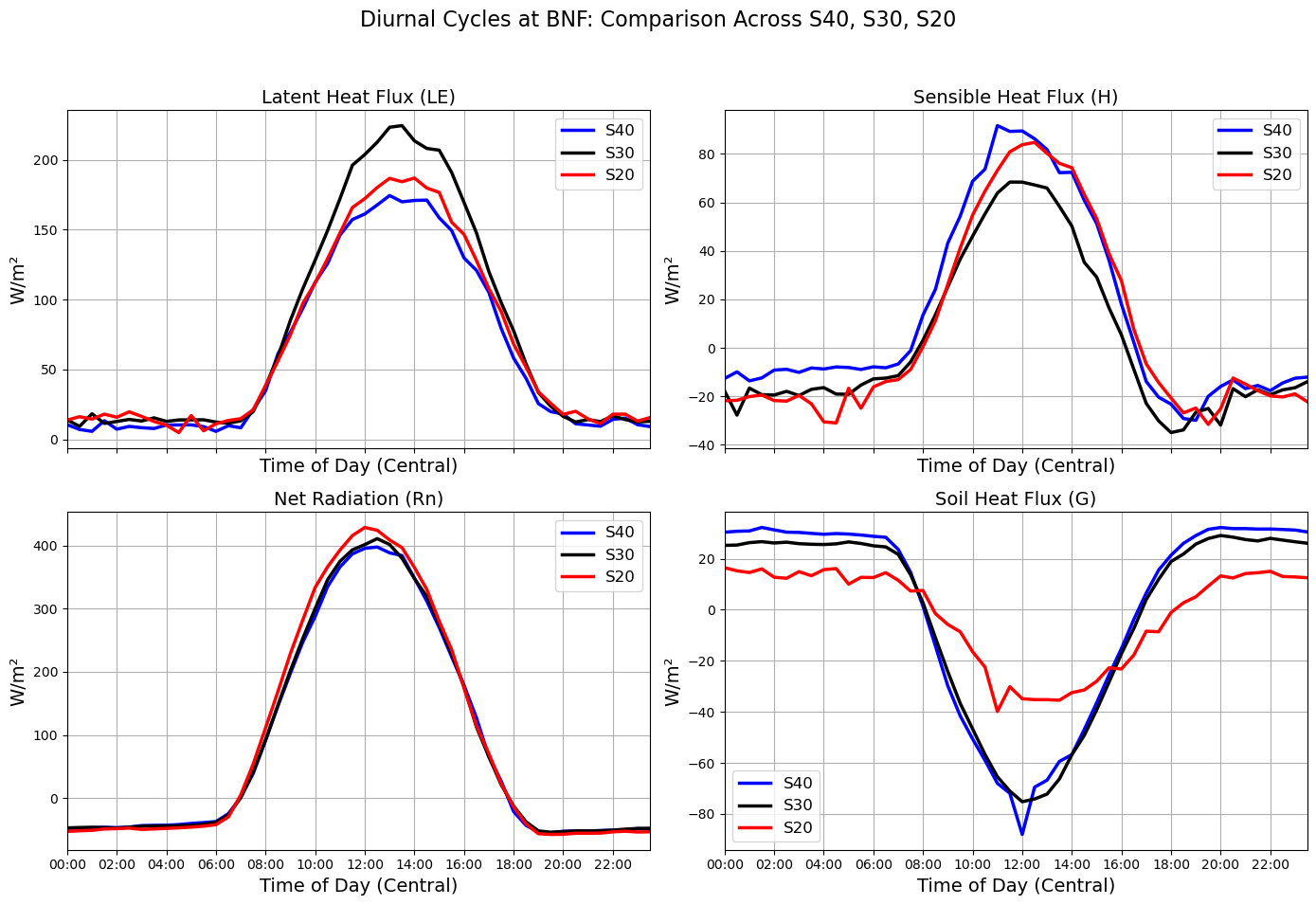
fig, axs = plt.subplots(2, 2, figsize=(14, 10), sharex=True)
axs = axs.flatten()
# Site styles: solid lines, different colors
site_styles = {
'S40': {'color': 'blue', 'label': 'S40'},
'S30': {'color': 'black', 'label': 'S30'},
'S20': {'color': 'red', 'label': 'S20'}
}
lw = 2.5
x = time_objects
# LE
axs[0].plot(x, le_avg_s40.values, linestyle='-', linewidth=lw, **site_styles['S40'])
axs[0].plot(x, le_avg_s30.values, linestyle='-', linewidth=lw, **site_styles['S30'])
axs[0].plot(x, le_avg_s20.values, linestyle='-', linewidth=lw, **site_styles['S20'])
axs[0].set_title("Latent Heat Flux (LE)", fontsize=14)
axs[0].legend(fontsize=12)
axs[0].grid(True)
# H
axs[1].plot(x, h_avg_s40.values, linestyle='-', linewidth=lw, **site_styles['S40'])
axs[1].plot(x, h_avg_s30.values, linestyle='-', linewidth=lw, **site_styles['S30'])
axs[1].plot(x, h_avg_s20.values, linestyle='-', linewidth=lw, **site_styles['S20'])
axs[1].set_title("Sensible Heat Flux (H)", fontsize=14)
axs[1].legend(fontsize=12)
axs[1].grid(True)
# Rn
axs[2].plot(x, rn_avg_s40.values, linestyle='-', linewidth=lw, **site_styles['S40'])
axs[2].plot(x, rn_avg_s30.values, linestyle='-', linewidth=lw, **site_styles['S30'])
axs[2].plot(x, rn_avg_s20.values, linestyle='-', linewidth=lw, **site_styles['S20'])
axs[2].set_title("Net Radiation (Rn)", fontsize=14)
axs[2].legend(fontsize=12)
axs[2].grid(True)
# G
axs[3].plot(x, g_avg_s40.values, linestyle='-', linewidth=lw, **site_styles['S40'])
axs[3].plot(x, g_avg_s30.values, linestyle='-', linewidth=lw, **site_styles['S30'])
axs[3].plot(x, g_avg_s20.values, linestyle='-', linewidth=lw, **site_styles['S20'])
axs[3].set_title("Soil Heat Flux (G)", fontsize=14)
axs[3].legend(fontsize=12)
axs[3].grid(True)
# Shared X-axis formatting
for ax in axs:
ax.set_xlim([x[0], x[-1]])
ax.xaxis.set_major_formatter(mdates.DateFormatter('%H:%M'))
ax.xaxis.set_major_locator(mdates.HourLocator(interval=2))
ax.set_xlabel("Time of Day (Central)", fontsize=14)
ax.set_ylabel("W/m²", fontsize=14)
plt.suptitle("Diurnal Cycles at BNF: Comparison Across S40, S30, S20", fontsize=16)
plt.tight_layout(rect=[0, 0.03, 1, 0.95])
plt.show()