Land Atmosphere Interactions

import act
import numpy as np
import xarray as xr
import matplotlib.pyplot as plt
from scipy.stats import linregress
import matplotlib.colors as colors
import pandas as pd
import matplotlib.dates as mdates

# Set your username and token here!
username = 'sanielson'
token = '467abc05f4c61fde'

# Set the datastream and start/enddates
datastream_sebs = 'bnfsebsS40.b1'
startdate = '2025-02-07'
enddate = '2025-04-30T23:59:59'

# Use ACT to easily download the data.  Watch for the data citation!  Show some support
# for ARM's instrument experts and cite their data if you use it in a publication
result_sebs = act.discovery.download_arm_data(username, token, datastream_sebs, startdate, enddate)

datastream_ecor = 'bnfecorsfS40.b1'
result_ecor = act.discovery.download_arm_data(username, token, datastream_ecor, startdate, enddate)

datastream_sirs = 'bnfsirsS40.b1'
result_sirs = act.discovery.download_arm_data(username, token, datastream_sirs, startdate, enddate)

[DOWNLOADING] bnfsebsS40.b1.20250401.000000.cdf
[DOWNLOADING] bnfsebsS40.b1.20250307.000000.cdf
[DOWNLOADING] bnfsebsS40.b1.20250326.000000.cdf
[DOWNLOADING] bnfsebsS40.b1.20250226.000000.cdf
[DOWNLOADING] bnfsebsS40.b1.20250213.000000.cdf
[DOWNLOADING] bnfsebsS40.b1.20250425.000000.cdf
[DOWNLOADING] bnfsebsS40.b1.20250302.000000.cdf
[DOWNLOADING] bnfsebsS40.b1.20250328.000000.cdf
[DOWNLOADING] bnfsebsS40.b1.20250430.000000.cdf
[DOWNLOADING] bnfsebsS40.b1.20250416.000000.cdf
[DOWNLOADING] bnfsebsS40.b1.20250315.000000.cdf
[DOWNLOADING] bnfsebsS40.b1.20250410.000000.cdf
[DOWNLOADING] bnfsebsS40.b1.20250324.000000.cdf
[DOWNLOADING] bnfsebsS40.b1.20250217.000000.cdf
[DOWNLOADING] bnfsebsS40.b1.20250304.000000.cdf
[DOWNLOADING] bnfsebsS40.b1.20250216.000000.cdf
[DOWNLOADING] bnfsebsS40.b1.20250331.000000.cdf
[DOWNLOADING] bnfsebsS40.b1.20250225.000000.cdf
[DOWNLOADING] bnfsebsS40.b1.20250406.000000.cdf
[DOWNLOADING] bnfsebsS40.b1.20250212.000000.cdf
[DOWNLOADING] bnfsebsS40.b1.20250219.000000.cdf
[DOWNLOADING] bnfsebsS40.b1.20250424.000000.cdf
[DOWNLOADING] bnfsebsS40.b1.20250426.000000.cdf
[DOWNLOADING] bnfsebsS40.b1.20250208.000000.cdf
[DOWNLOADING] bnfsebsS40.b1.20250221.000000.cdf
[DOWNLOADING] bnfsebsS40.b1.20250311.000000.cdf
[DOWNLOADING] bnfsebsS40.b1.20250414.000000.cdf
[DOWNLOADING] bnfsebsS40.b1.20250428.000000.cdf
[DOWNLOADING] bnfsebsS40.b1.20250301.000000.cdf
[DOWNLOADING] bnfsebsS40.b1.20250310.000000.cdf
[DOWNLOADING] bnfsebsS40.b1.20250223.000000.cdf
[DOWNLOADING] bnfsebsS40.b1.20250321.000000.cdf
[DOWNLOADING] bnfsebsS40.b1.20250330.000000.cdf
[DOWNLOADING] bnfsebsS40.b1.20250210.000000.cdf
[DOWNLOADING] bnfsebsS40.b1.20250227.000000.cdf
[DOWNLOADING] bnfsebsS40.b1.20250325.000000.cdf
[DOWNLOADING] bnfsebsS40.b1.20250211.000000.cdf
[DOWNLOADING] bnfsebsS40.b1.20250412.000000.cdf
[DOWNLOADING] bnfsebsS40.b1.20250207.000000.cdf
[DOWNLOADING] bnfsebsS40.b1.20250409.000000.cdf
[DOWNLOADING] bnfsebsS40.b1.20250411.000000.cdf
[DOWNLOADING] bnfsebsS40.b1.20250417.000000.cdf
[DOWNLOADING] bnfsebsS40.b1.20250419.000000.cdf
[DOWNLOADING] bnfsebsS40.b1.20250408.000000.cdf
[DOWNLOADING] bnfsebsS40.b1.20250418.000000.cdf
[DOWNLOADING] bnfsebsS40.b1.20250319.000000.cdf
[DOWNLOADING] bnfsebsS40.b1.20250309.000000.cdf
[DOWNLOADING] bnfsebsS40.b1.20250421.000000.cdf
[DOWNLOADING] bnfsebsS40.b1.20250402.000000.cdf
[DOWNLOADING] bnfsebsS40.b1.20250228.000000.cdf
[DOWNLOADING] bnfsebsS40.b1.20250420.000000.cdf
[DOWNLOADING] bnfsebsS40.b1.20250427.000000.cdf
[DOWNLOADING] bnfsebsS40.b1.20250415.000000.cdf
[DOWNLOADING] bnfsebsS40.b1.20250320.000000.cdf
[DOWNLOADING] bnfsebsS40.b1.20250322.000000.cdf
[DOWNLOADING] bnfsebsS40.b1.20250303.000000.cdf
[DOWNLOADING] bnfsebsS40.b1.20250215.000000.cdf
[DOWNLOADING] bnfsebsS40.b1.20250405.000000.cdf
[DOWNLOADING] bnfsebsS40.b1.20250403.000000.cdf
[DOWNLOADING] bnfsebsS40.b1.20250220.000000.cdf
[DOWNLOADING] bnfsebsS40.b1.20250308.000000.cdf
[DOWNLOADING] bnfsebsS40.b1.20250222.000000.cdf
[DOWNLOADING] bnfsebsS40.b1.20250429.000000.cdf
[DOWNLOADING] bnfsebsS40.b1.20250314.000000.cdf
[DOWNLOADING] bnfsebsS40.b1.20250329.000000.cdf
[DOWNLOADING] bnfsebsS40.b1.20250318.000000.cdf
[DOWNLOADING] bnfsebsS40.b1.20250327.000000.cdf
[DOWNLOADING] bnfsebsS40.b1.20250323.000000.cdf
[DOWNLOADING] bnfsebsS40.b1.20250312.000000.cdf
[DOWNLOADING] bnfsebsS40.b1.20250313.000000.cdf
[DOWNLOADING] bnfsebsS40.b1.20250404.000000.cdf
[DOWNLOADING] bnfsebsS40.b1.20250305.000000.cdf
[DOWNLOADING] bnfsebsS40.b1.20250317.000000.cdf
[DOWNLOADING] bnfsebsS40.b1.20250209.000000.cdf
[DOWNLOADING] bnfsebsS40.b1.20250423.000000.cdf
[DOWNLOADING] bnfsebsS40.b1.20250218.000000.cdf
[DOWNLOADING] bnfsebsS40.b1.20250306.000000.cdf
[DOWNLOADING] bnfsebsS40.b1.20250316.000000.cdf
[DOWNLOADING] bnfsebsS40.b1.20250224.000000.cdf
[DOWNLOADING] bnfsebsS40.b1.20250214.000000.cdf
[DOWNLOADING] bnfsebsS40.b1.20250413.000000.cdf
[DOWNLOADING] bnfsebsS40.b1.20250407.000000.cdf
[DOWNLOADING] bnfsebsS40.b1.20250422.000000.cdf

If you use these data to prepare a publication, please cite:

Sullivan, R., Keeler, E., Pal, S., & Kyrouac, J. Surface Energy Balance System
(SEBS), 2025-02-07 to 2025-04-30, Bankhead National Forest, AL, USA; Long-term
Mobile Facility (BNF), Bankhead National Forest, AL, Supplemental facility at
Double Springs (S40). Atmospheric Radiation Measurement (ARM) User Facility.
https://doi.org/10.5439/1984921

[DOWNLOADING] bnfecorsfS40.b1.20250409.000000.nc
[DOWNLOADING] bnfecorsfS40.b1.20250411.000000.nc
[DOWNLOADING] bnfecorsfS40.b1.20250429.000000.nc
[DOWNLOADING] bnfecorsfS40.b1.20250226.000000.nc
[DOWNLOADING] bnfecorsfS40.b1.20250404.000000.nc
[DOWNLOADING] bnfecorsfS40.b1.20250426.000000.nc
[DOWNLOADING] bnfecorsfS40.b1.20250304.000000.nc
[DOWNLOADING] bnfecorsfS40.b1.20250309.000000.nc
[DOWNLOADING] bnfecorsfS40.b1.20250413.000000.nc
[DOWNLOADING] bnfecorsfS40.b1.20250422.000000.nc
[DOWNLOADING] bnfecorsfS40.b1.20250417.000000.nc
[DOWNLOADING] bnfecorsfS40.b1.20250212.233000.nc
[DOWNLOADING] bnfecorsfS40.b1.20250408.000000.nc
[DOWNLOADING] bnfecorsfS40.b1.20250406.000000.nc
[DOWNLOADING] bnfecorsfS40.b1.20250217.000000.nc
[DOWNLOADING] bnfecorsfS40.b1.20250307.000000.nc
[DOWNLOADING] bnfecorsfS40.b1.20250410.000000.nc
[DOWNLOADING] bnfecorsfS40.b1.20250424.000000.nc
[DOWNLOADING] bnfecorsfS40.b1.20250312.000000.nc
[DOWNLOADING] bnfecorsfS40.b1.20250412.000000.nc
[DOWNLOADING] bnfecorsfS40.b1.20250419.000000.nc
[DOWNLOADING] bnfecorsfS40.b1.20250308.000000.nc
[DOWNLOADING] bnfecorsfS40.b1.20250228.000000.nc
[DOWNLOADING] bnfecorsfS40.b1.20250225.000000.nc
[DOWNLOADING] bnfecorsfS40.b1.20250302.000000.nc
[DOWNLOADING] bnfecorsfS40.b1.20250218.000000.nc
[DOWNLOADING] bnfecorsfS40.b1.20250213.000000.nc
[DOWNLOADING] bnfecorsfS40.b1.20250305.000000.nc
[DOWNLOADING] bnfecorsfS40.b1.20250415.000000.nc
[DOWNLOADING] bnfecorsfS40.b1.20250222.000000.nc
[DOWNLOADING] bnfecorsfS40.b1.20250430.000000.nc
[DOWNLOADING] bnfecorsfS40.b1.20250307.233000.nc
[DOWNLOADING] bnfecorsfS40.b1.20250310.000000.nc
[DOWNLOADING] bnfecorsfS40.b1.20250219.000000.nc
[DOWNLOADING] bnfecorsfS40.b1.20250208.000000.nc
[DOWNLOADING] bnfecorsfS40.b1.20250214.000000.nc
[DOWNLOADING] bnfecorsfS40.b1.20250220.000000.nc
[DOWNLOADING] bnfecorsfS40.b1.20250211.000000.nc
[DOWNLOADING] bnfecorsfS40.b1.20250221.000000.nc
[DOWNLOADING] bnfecorsfS40.b1.20250209.000000.nc
[DOWNLOADING] bnfecorsfS40.b1.20250223.000000.nc
[DOWNLOADING] bnfecorsfS40.b1.20250405.000000.nc
[DOWNLOADING] bnfecorsfS40.b1.20250418.000000.nc
[DOWNLOADING] bnfecorsfS40.b1.20250224.000000.nc
[DOWNLOADING] bnfecorsfS40.b1.20250414.000000.nc
[DOWNLOADING] bnfecorsfS40.b1.20250416.000000.nc
[DOWNLOADING] bnfecorsfS40.b1.20250227.000000.nc
[DOWNLOADING] bnfecorsfS40.b1.20250427.000000.nc
[DOWNLOADING] bnfecorsfS40.b1.20250403.160000.nc
[DOWNLOADING] bnfecorsfS40.b1.20250420.000000.nc
[DOWNLOADING] bnfecorsfS40.b1.20250303.000000.nc
[DOWNLOADING] bnfecorsfS40.b1.20250313.000000.nc
[DOWNLOADING] bnfecorsfS40.b1.20250207.000000.nc
[DOWNLOADING] bnfecorsfS40.b1.20250423.000000.nc
[DOWNLOADING] bnfecorsfS40.b1.20250212.000000.nc
[DOWNLOADING] bnfecorsfS40.b1.20250425.000000.nc
[DOWNLOADING] bnfecorsfS40.b1.20250311.000000.nc
[DOWNLOADING] bnfecorsfS40.b1.20250301.000000.nc
[DOWNLOADING] bnfecorsfS40.b1.20250306.000000.nc
[DOWNLOADING] bnfecorsfS40.b1.20250215.000000.nc
[DOWNLOADING] bnfecorsfS40.b1.20250421.000000.nc
[DOWNLOADING] bnfecorsfS40.b1.20250210.000000.nc
[DOWNLOADING] bnfecorsfS40.b1.20250216.000000.nc
[DOWNLOADING] bnfecorsfS40.b1.20250407.000000.nc
[DOWNLOADING] bnfecorsfS40.b1.20250428.000000.nc

If you use these data to prepare a publication, please cite:

Sullivan, R., Cook, D., Shi, Y., Keeler, E., & Pal, S. Eddy Correlation Flux
Measurement System (ECORSF), 2025-02-07 to 2025-04-30, Bankhead National Forest,
AL, USA; Long-term Mobile Facility (BNF), Bankhead National Forest, AL,
Supplemental facility at Double Springs (S40). Atmospheric Radiation Measurement
(ARM) User Facility. https://doi.org/10.5439/1494128

[DOWNLOADING] bnfsirsS40.b1.20250314.000000.nc
[DOWNLOADING] bnfsirsS40.b1.20250213.000000.nc
[DOWNLOADING] bnfsirsS40.b1.20250421.000000.nc
[DOWNLOADING] bnfsirsS40.b1.20250324.000000.nc
[DOWNLOADING] bnfsirsS40.b1.20250317.000000.nc
[DOWNLOADING] bnfsirsS40.b1.20250218.000000.nc
[DOWNLOADING] bnfsirsS40.b1.20250426.000000.nc
[DOWNLOADING] bnfsirsS40.b1.20250420.000000.nc
[DOWNLOADING] bnfsirsS40.b1.20250313.000000.nc
[DOWNLOADING] bnfsirsS40.b1.20250404.000000.nc
[DOWNLOADING] bnfsirsS40.b1.20250304.000000.nc
[DOWNLOADING] bnfsirsS40.b1.20250208.000000.nc
[DOWNLOADING] bnfsirsS40.b1.20250318.000000.nc
[DOWNLOADING] bnfsirsS40.b1.20250309.000000.nc
[DOWNLOADING] bnfsirsS40.b1.20250419.000000.nc
[DOWNLOADING] bnfsirsS40.b1.20250329.000000.nc
[DOWNLOADING] bnfsirsS40.b1.20250215.000000.nc
[DOWNLOADING] bnfsirsS40.b1.20250224.000000.nc
[DOWNLOADING] bnfsirsS40.b1.20250321.000000.nc
[DOWNLOADING] bnfsirsS40.b1.20250411.000000.nc
[DOWNLOADING] bnfsirsS40.b1.20250414.000000.nc
[DOWNLOADING] bnfsirsS40.b1.20250402.000000.nc
[DOWNLOADING] bnfsirsS40.b1.20250228.000000.nc
[DOWNLOADING] bnfsirsS40.b1.20250310.000000.nc
[DOWNLOADING] bnfsirsS40.b1.20250320.000000.nc
[DOWNLOADING] bnfsirsS40.b1.20250216.000000.nc
[DOWNLOADING] bnfsirsS40.b1.20250312.000000.nc
[DOWNLOADING] bnfsirsS40.b1.20250210.000000.nc
[DOWNLOADING] bnfsirsS40.b1.20250221.000000.nc
[DOWNLOADING] bnfsirsS40.b1.20250311.000000.nc
[DOWNLOADING] bnfsirsS40.b1.20250303.000000.nc
[DOWNLOADING] bnfsirsS40.b1.20250406.000000.nc
[DOWNLOADING] bnfsirsS40.b1.20250217.000000.nc
[DOWNLOADING] bnfsirsS40.b1.20250330.000000.nc
[DOWNLOADING] bnfsirsS40.b1.20250323.000000.nc
[DOWNLOADING] bnfsirsS40.b1.20250424.000000.nc
[DOWNLOADING] bnfsirsS40.b1.20250428.000000.nc
[DOWNLOADING] bnfsirsS40.b1.20250212.000000.nc
[DOWNLOADING] bnfsirsS40.b1.20250319.000000.nc
[DOWNLOADING] bnfsirsS40.b1.20250326.000000.nc
[DOWNLOADING] bnfsirsS40.b1.20250427.000000.nc
[DOWNLOADING] bnfsirsS40.b1.20250207.120000.nc
[DOWNLOADING] bnfsirsS40.b1.20250429.000000.nc
[DOWNLOADING] bnfsirsS40.b1.20250225.000000.nc
[DOWNLOADING] bnfsirsS40.b1.20250214.000000.nc
[DOWNLOADING] bnfsirsS40.b1.20250401.000000.nc
[DOWNLOADING] bnfsirsS40.b1.20250416.000000.nc
[DOWNLOADING] bnfsirsS40.b1.20250322.000000.nc
[DOWNLOADING] bnfsirsS40.b1.20250305.000000.nc
[DOWNLOADING] bnfsirsS40.b1.20250425.000000.nc
[DOWNLOADING] bnfsirsS40.b1.20250413.000000.nc
[DOWNLOADING] bnfsirsS40.b1.20250417.000000.nc
[DOWNLOADING] bnfsirsS40.b1.20250403.000000.nc
[DOWNLOADING] bnfsirsS40.b1.20250220.000000.nc
[DOWNLOADING] bnfsirsS40.b1.20250410.000000.nc
[DOWNLOADING] bnfsirsS40.b1.20250308.000000.nc
[DOWNLOADING] bnfsirsS40.b1.20250207.110000.nc
[DOWNLOADING] bnfsirsS40.b1.20250307.000000.nc
[DOWNLOADING] bnfsirsS40.b1.20250301.000000.nc
[DOWNLOADING] bnfsirsS40.b1.20250331.000000.nc
[DOWNLOADING] bnfsirsS40.b1.20250211.000000.nc
[DOWNLOADING] bnfsirsS40.b1.20250409.000000.nc
[DOWNLOADING] bnfsirsS40.b1.20250430.000000.nc
[DOWNLOADING] bnfsirsS40.b1.20250207.000000.nc
[DOWNLOADING] bnfsirsS40.b1.20250315.000000.nc
[DOWNLOADING] bnfsirsS40.b1.20250226.000000.nc
[DOWNLOADING] bnfsirsS40.b1.20250219.000000.nc
[DOWNLOADING] bnfsirsS40.b1.20250222.000000.nc
[DOWNLOADING] bnfsirsS40.b1.20250423.000000.nc
[DOWNLOADING] bnfsirsS40.b1.20250327.000000.nc
[DOWNLOADING] bnfsirsS40.b1.20250306.000000.nc
[DOWNLOADING] bnfsirsS40.b1.20250408.000000.nc
[DOWNLOADING] bnfsirsS40.b1.20250325.000000.nc
[DOWNLOADING] bnfsirsS40.b1.20250418.000000.nc
[DOWNLOADING] bnfsirsS40.b1.20250415.000000.nc
[DOWNLOADING] bnfsirsS40.b1.20250328.000000.nc
[DOWNLOADING] bnfsirsS40.b1.20250307.010000.nc
[DOWNLOADING] bnfsirsS40.b1.20250227.000000.nc
[DOWNLOADING] bnfsirsS40.b1.20250412.000000.nc
[DOWNLOADING] bnfsirsS40.b1.20250316.000000.nc
[DOWNLOADING] bnfsirsS40.b1.20250407.150000.nc
[DOWNLOADING] bnfsirsS40.b1.20250405.000000.nc
[DOWNLOADING] bnfsirsS40.b1.20250406.100000.nc
[DOWNLOADING] bnfsirsS40.b1.20250209.000000.nc
[DOWNLOADING] bnfsirsS40.b1.20250422.000000.nc
[DOWNLOADING] bnfsirsS40.b1.20250223.000000.nc
[DOWNLOADING] bnfsirsS40.b1.20250302.000000.nc

If you use these data to prepare a publication, please cite:

Sengupta, M., Xie, Y., Jaker, S., Yang, J., Reda, I., Andreas, A., Habte, A., &
Shi, Y. Solar and Infrared Radiation Station for Downwelling and Upwelling
Radiation (SIRS), 2025-02-07 to 2025-04-30, Bankhead National Forest, AL, USA;
Long-term Mobile Facility (BNF), Bankhead National Forest, AL, Supplemental
facility at Double Springs (S40). Atmospheric Radiation Measurement (ARM) User
Facility. https://doi.org/10.5439/1475460

# Let's read in the data using ACT and check out the data
ds_sebs = act.io.read_arm_netcdf(result_sebs)
ds_sebs

#ECOR has sensible and latent heat flux together
ds_ecor = act.io.read_arm_netcdf(result_ecor)
ds_ecor

# Let's read in the data using ACT and check out the data
ds_sirs = act.io.read_arm_netcdf(result_sirs)
ds_sirs

ds_sirs.clean.cleanup()

down_long = 'down_long_hemisp1'
up_long = 'up_long_hemisp'
down_short = 'down_short_hemisp'
up_short = 'up_short_hemisp'

display = act.plotting.TimeSeriesDisplay(ds_sirs, figsize=(15, 10))

# Plot up the variable in the plots
display.plot(down_long, subplot_index=(0,))
display.plot(up_long, subplot_index=(0,))
display.plot(down_short, subplot_index=(0,))
display.plot(up_short, subplot_index=(0,))

# Plot up a day/night background
display.day_night_background(subplot_index=(0,))

# Plot up a day/night background
#display.day_night_background(subplot_index=(0,))
plt.show()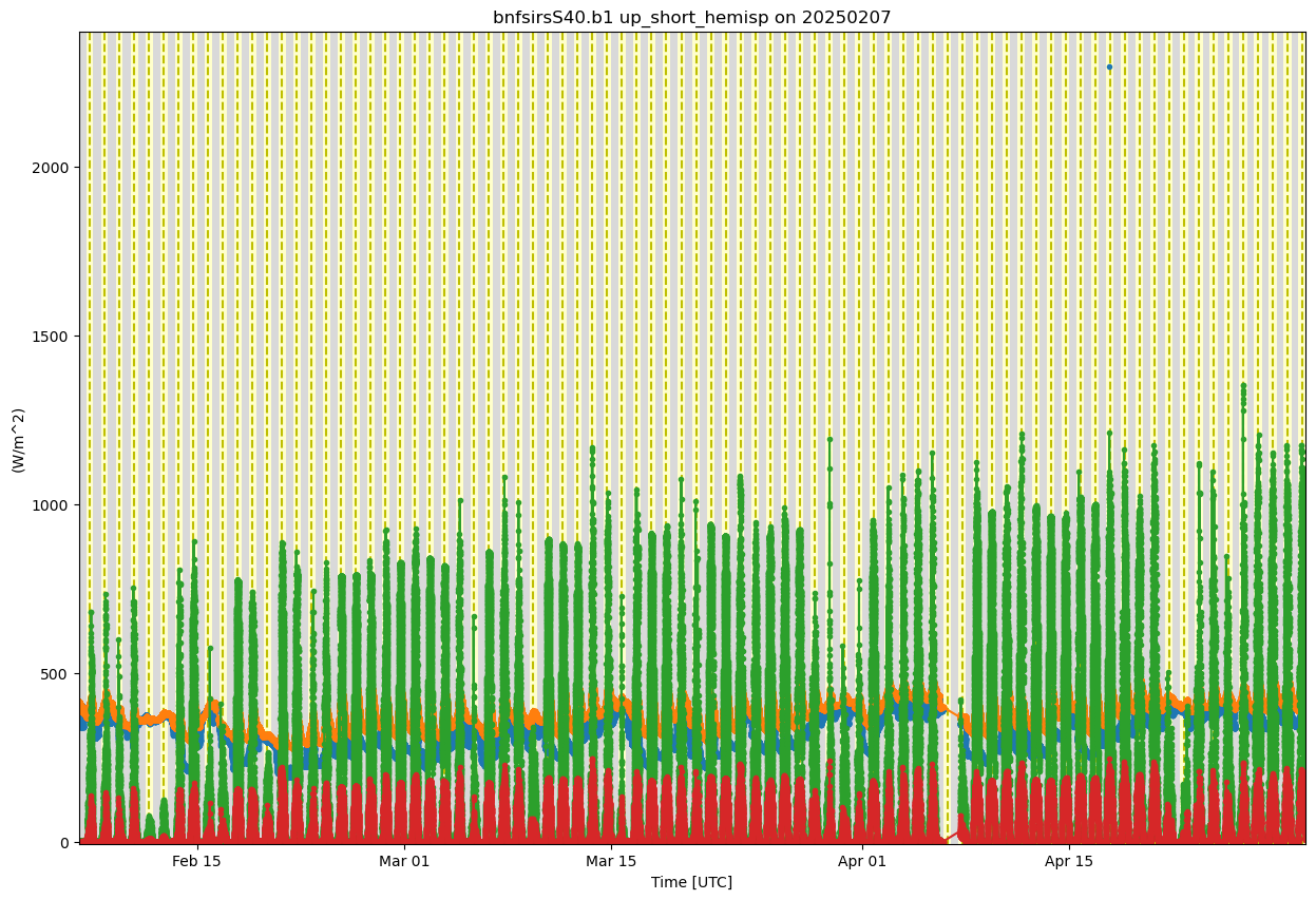

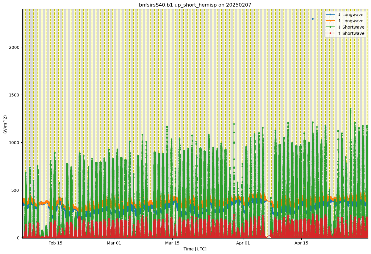
display = act.plotting.TimeSeriesDisplay(ds_sirs, figsize=(15, 10))

# Plot each variable with a label
display.plot(down_long, subplot_index=(0,), label='↓ Longwave')
display.plot(up_long, subplot_index=(0,), label='↑ Longwave')
display.plot(down_short, subplot_index=(0,), label='↓ Shortwave')
display.plot(up_short, subplot_index=(0,), label='↑ Shortwave')

# Add day/night background
display.day_night_background(subplot_index=(0,))

# Show legend manually
display.axes[0].legend(loc='upper right')

plt.show()

net_radiation = (ds_sirs['down_long_hemisp1'] - ds_sirs['up_long_hemisp']) + (ds_sirs['down_short_hemisp'] - ds_sirs['up_short_hemisp'])

#net radiation calculations
net_radiation.plot()
plt.title('Net Radiation')
plt.ylabel('Radiation')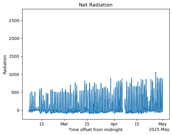

ds_sebs.clean.cleanup()

soil_flux = 'surface_soil_heat_flux_avg'

display = act.plotting.TimeSeriesDisplay(ds_sebs, figsize=(15, 10))

# Plot up the variable in the plots
display.plot(soil_flux, subplot_index=(0,))

# Plot up a day/night background
display.day_night_background(subplot_index=(0,))

plt.show()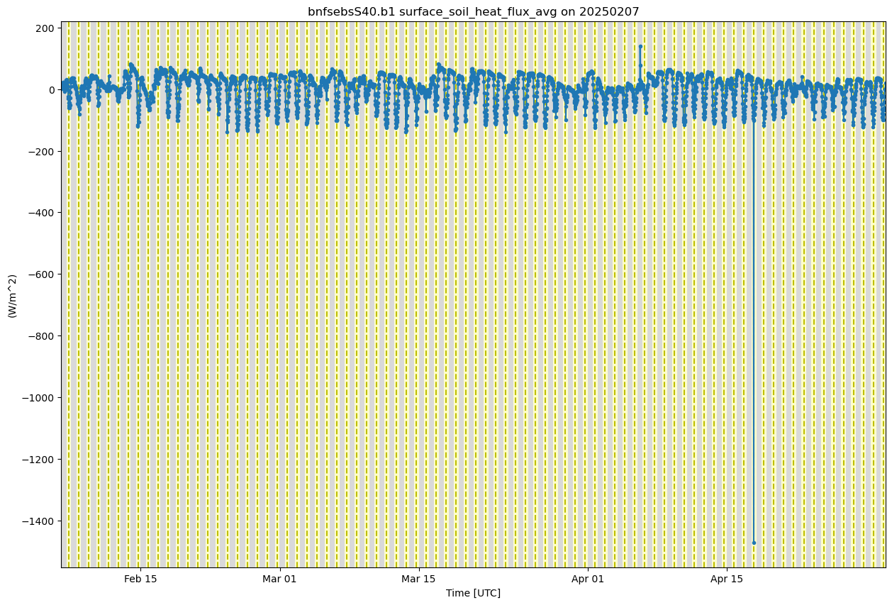

avail_e = net_radiation - ds_sebs['surface_soil_heat_flux_avg']

#net radiation calculations
avail_e.plot()
plt.title('Net Radiation')
plt.ylabel('Radiation')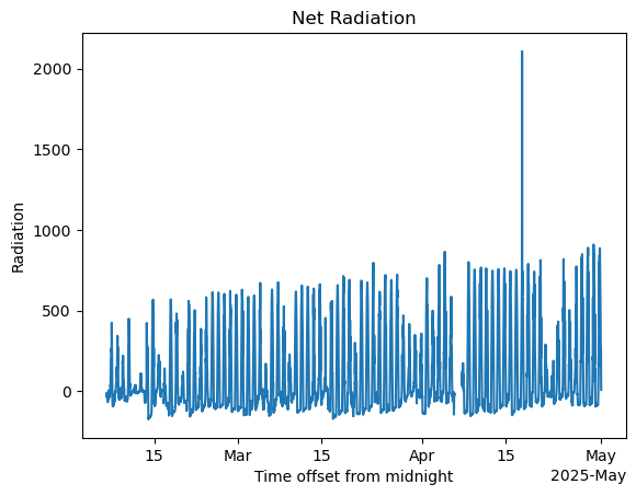

ds_ecor.clean.cleanup()

sensible_flux = 'sensible_heat_flux'
latent_flux = 'latent_flux'

display = act.plotting.TimeSeriesDisplay(ds_ecor, figsize=(15, 10))

# Plot up the variable in the plots
display.plot(sensible_flux, subplot_index=(0,), color='red')
display.plot(latent_flux, subplot_index=(0,), color='blue')

# Plot up a day/night background
display.day_night_background(subplot_index=(0,))

# Plot up a day/night background
#display.day_night_background(subplot_index=(0,))
plt.show()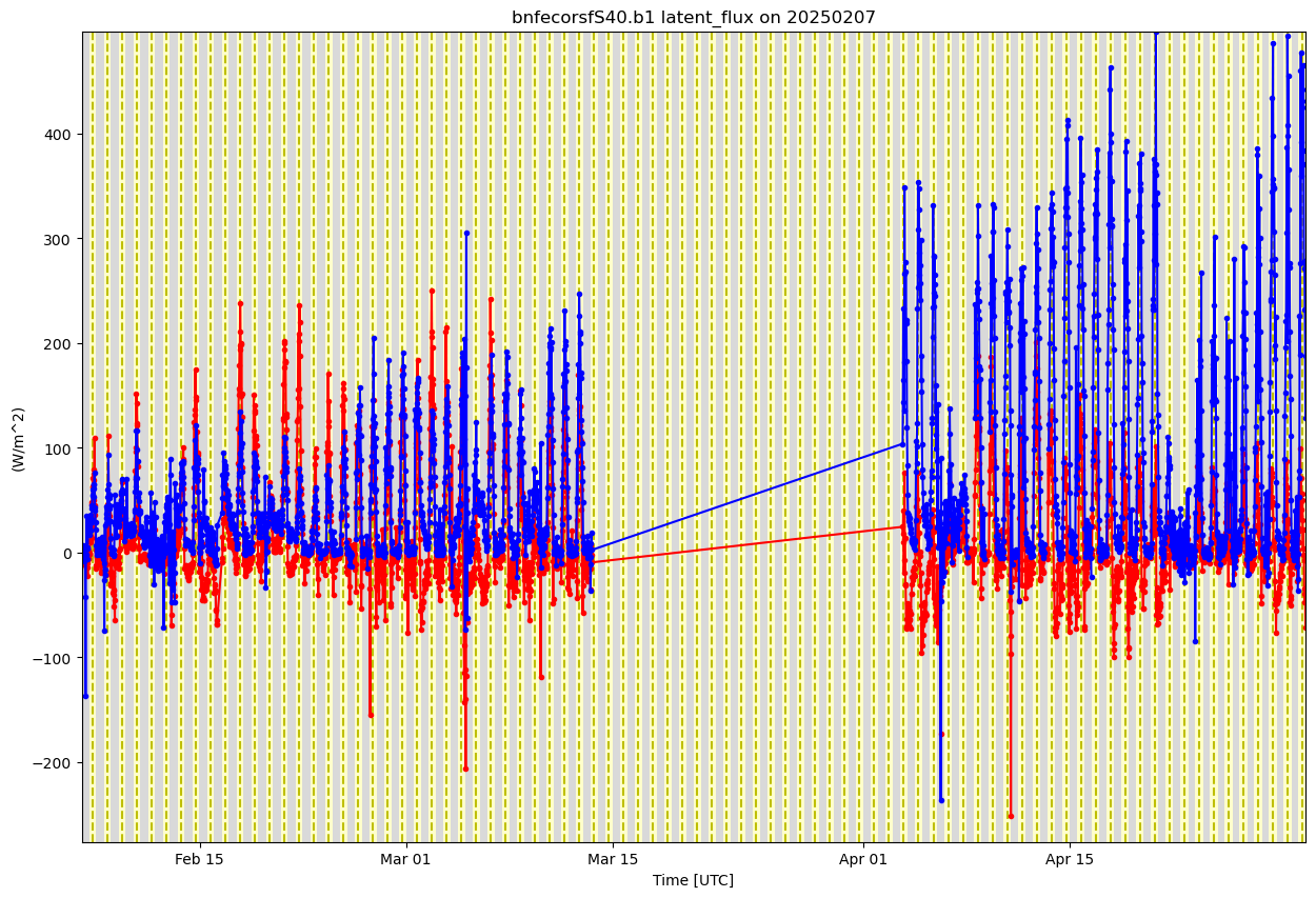

turb_flux = ds_ecor['sensible_heat_flux'] + ds_ecor['latent_flux']

#net radiation calculations
turb_flux.plot()
plt.title('Turbulent Flux')
plt.ylabel('Radiation')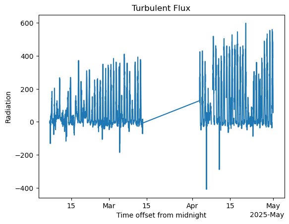

turb_flux_aligned, avail_e_aligned = xr.align(turb_flux, avail_e, join = 'inner')

# Convert to numpy arrays
x = avail_e_aligned.values
y = turb_flux_aligned.values
# Remove NaNs
mask = ~np.isnan(x) & ~np.isnan(y)
x = x[mask]
y = y[mask]
# Fit regression
from scipy.stats import linregress
slope, intercept, r_value, p_value, std_err = linregress(x, y)
# Sort x for clean line plot
sort_idx = np.argsort(x)
x_sorted = x[sort_idx]
y_fit = slope * x_sorted + intercept
# Plot
import matplotlib.pyplot as plt
plt.figure(figsize=(8,6))
plt.scatter(x, y, alpha=0.6, label='Data')
plt.plot(x_sorted, y_fit, 'r-', label=f'Fit: y = {slope:.2f}x + {intercept:.1f}')
plt.plot([x.min(), x.max()], [x.min(), x.max()], 'k--', label='1:1 line')
plt.xlabel("Available Energy (Rn - G) [W/m²]")
plt.ylabel("Turbulent Flux (H + LE) [W/m²]")
plt.title("Energy Balance Closure at BNF")
plt.legend()
plt.grid(True)
plt.show()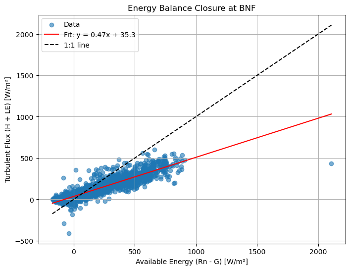

# --- Step 1: Timezone-aware time-of-day coordinate ---
def add_time_of_day(da):
    utc_times = pd.to_datetime(da.time.values).tz_localize('UTC')
    central_times = utc_times.tz_convert('US/Central')
    rounded = central_times.floor('30min')
    time_of_day_strs = xr.DataArray(rounded.strftime('%H:%M'), coords={'time': da.time}, dims='time')
    return da.assign_coords(time_of_day=time_of_day_strs)

# --- Step 2: Assign to each variable ---
le_td = add_time_of_day(ds_ecor['latent_flux'])
h_td  = add_time_of_day(ds_ecor['sensible_heat_flux'])
rn_td = add_time_of_day(net_radiation)
g_td  = add_time_of_day(ds_sebs['surface_soil_heat_flux_avg'])

# --- Step 3: Group by time-of-day and average ---
le_avg = le_td.groupby('time_of_day').mean('time')
h_avg  = h_td.groupby('time_of_day').mean('time')
rn_avg = rn_td.groupby('time_of_day').mean('time')
g_avg  = g_td.groupby('time_of_day').mean('time')

# --- Step 4: Sort by time ---
def sort_by_time(da):
    parsed = pd.to_datetime(da.time_of_day.values, format='%H:%M')
    sort_idx = np.argsort(parsed)
    return da.isel(time_of_day=sort_idx)

le_avg = sort_by_time(le_avg)
h_avg  = sort_by_time(h_avg)
rn_avg = sort_by_time(rn_avg)
g_avg  = sort_by_time(g_avg)

# --- Step 5: Prepare time axis ---
time_objects = pd.to_datetime(le_avg.time_of_day.values, format='%H:%M')

# --- Step 6: Plot with CUD colors and thicker lines ---
# Color-blind–friendly colors (CUD palette)
colors = {
    'LE': '#E69F00',  # orange
    'H': '#56B4E9',   # sky blue
    'Rn': '#009E73',  # bluish green
    'G': '#D55E00'    # vermillion
}

plt.figure(figsize=(12, 6))
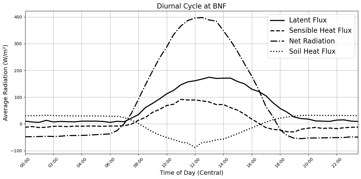
plt.plot(time_objects, le_avg.values, label='Latent Flux', color='black', linestyle='-', linewidth=2.5)
plt.plot(time_objects, h_avg.values, label='Sensible Heat Flux', color='black', linestyle='--', linewidth=2.5)
plt.plot(time_objects, rn_avg.values, label='Net Radiation', color='black', linestyle='-.', linewidth=2.5)
plt.plot(time_objects, g_avg.values, label='Soil Heat Flux', color='black', linestyle=':', linewidth=2.5)

# Format x-axis
ax = plt.gca()
ax.xaxis.set_major_formatter(mdates.DateFormatter('%H:%M'))
ax.xaxis.set_major_locator(mdates.HourLocator(interval=2))
plt.xlim([time_objects[0], time_objects[-1]])

plt.xlabel("Time of Day (Central)", fontsize=14)
plt.ylabel("Average Radiation (W/m²)", fontsize=14)
plt.title("Diurnal Cycle at BNF", fontsize=16)
plt.xticks(rotation=45)
plt.legend(fontsize=16)
plt.grid(True)
plt.tight_layout()
plt.show()

Land Atmosphere Interactions

S30 Total Radiation Saranielson

Land Atmosphere Interactions

Imports