We can run multidoppler analyses on the May 20, 2025 case where we have CSAPR2 (ARM) and NEXRAD (NOAA) precipitation radar data.
Imports
import pyart
import pydda
import glob
import pandas as pd
import xarray as xr
from datetime import timedelta
import matplotlib.pyplot as plt
Run Multidoppler Analyses using Pydda
We follow the instructions from the PyDDA user’s guide: https://
The data has been pre-gridded and cleaned (ie dealiased)
nexrad_grids = sorted(glob.glob("/data/project/ARM_Summer_School_2025/radar/dda/20250520/csapr2/*"))
csapr_grids = sorted(glob.glob("/data/project/ARM_Summer_School_2025/radar/dda/20250520/nexrad/*"))

_, sonde = pyart.io.read_arm_sonde("/data/project/ARM_Summer_School_2025/bnf/bnfsondewnpnM1.b1/bnfsondewnpnM1.b1.20250520.233000.cdf")
Configure matching times
Taking a look at the volume files, match the times
time_matching = {"2230": {"csapr": 3,
                          "nexrad": 0},
                 "2240": {"csapr": 4,
                          "nexrad": 2},
                 "2250": {"csapr": 5,
                          "nexrad": 4},
                 "2300": {"csapr": 6,
                          "nexrad": 6},
                 "2310": {"csapr": 7,
                          "nexrad": 8},
                 "2320": {"csapr": 8,
                          "nexrad": 10},
                }
def process_dda(nexrad_file, csapr_file, outfile):
"""
nexrad_file: str
File containing the nexrad data to be used for multidoppler analyses
csapr_file: str
File containing the csapr2 data to be used fo multidoppler analyses
outfile: str
File to output the grid to
"""
grid_nexrad = pydda.io.read_grid(nexrad_file)
grid_csapr = pydda.io.read_grid(csapr_file)
grid_csapr = pydda.initialization.make_constant_wind_field(grid_csapr,
(0.0, 0.0, 0.0),
vel_field='mean_doppler_velocity')
grids_out, _ = pydda.retrieval.get_dd_wind_field([grid_csapr, grid_nexrad],
Co=1,
Cm=500.,
Cx=1e-2,
Cy=1e-2,
Cz=1e-2,
frz=4000.0,
u_back=sonde.u_wind,
v_back=sonde.v_wind,
z_back=sonde.height,
refl_field='reflectivity',
wind_tol=0.5,
max_iterations=50,
filter_window=15,
filter_order=3,
engine='tensorflow')
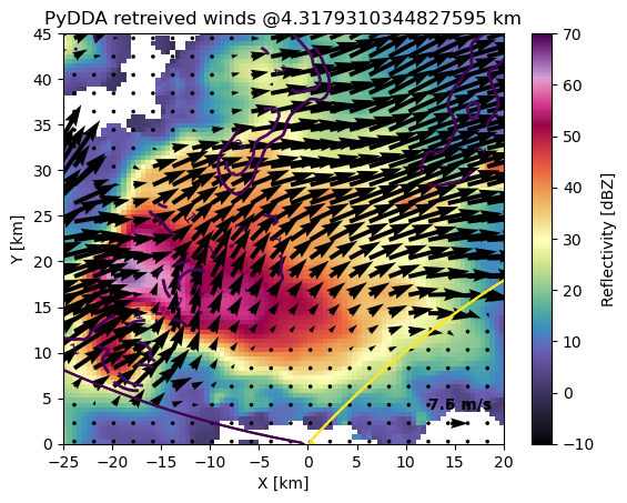
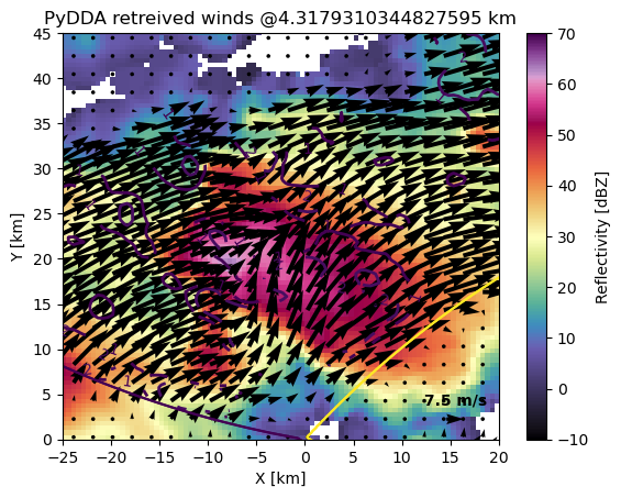
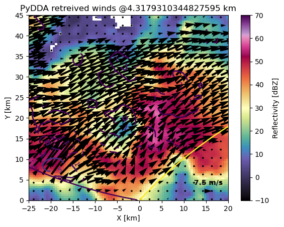
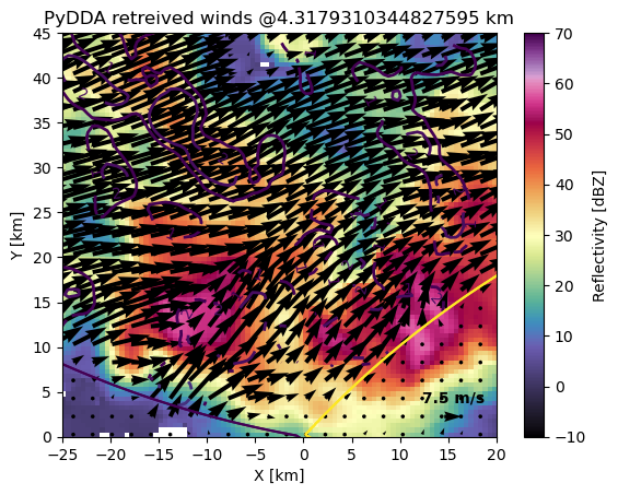
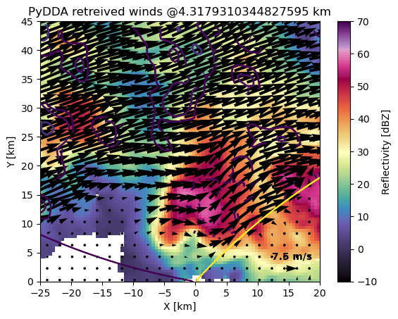
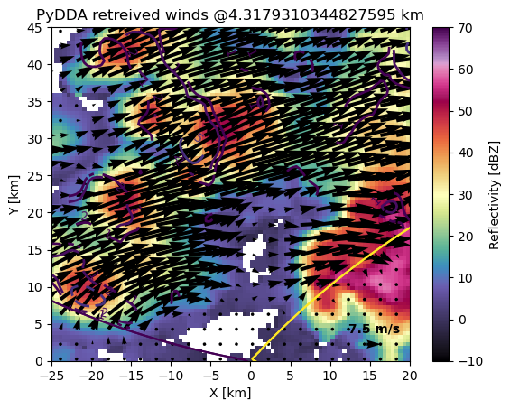
pydda.vis.plot_horiz_xsection_quiver(grids_out,
level=8,
cmap='ChaseSpectral',
vmin=-10,
vmax=70,
quiverkey_len=7.5,
background_field='reflectivity',
bg_grid_no=1,
w_vel_contours=[1, 2, 5, 10, 20, 30],
quiver_spacing_x_km=2.5,
quiver_spacing_y_km=2.5,
quiverkey_loc='bottom_right')
plt.ylim(0, 45)
plt.xlim(-25, 20)
plt.show()
plt.close()
out = grids_out[0]
out.to_netcdf(outfile)
print(outfile)
for time in time_matching:
    single_time = time_matching[time]
    process_dda(nexrad_grids[single_time["nexrad"]],
                csapr_grids[single_time["csapr"]],
                f"pydda-20250520{time}.nc")
ERROR! Session/line number was not unique in database. History logging moved to new session 341
Interpolating sounding to radar grid
Interpolated U field:
tf.Tensor(
[ nan 4.5307264 11.4344845 15.301979 21.562355 23.875206
26.482462 25.819971 28.538422 30. 30.381481 32.848923
33.17398 32.373234 27.429451 28.3827 30.325945 27.802431
21.681234 22.78611 25.718634 28.756817 26.373087 26.310108
25.113314 33.57475 34.139362 39.02031 30.191198 27.088177 ], shape=(30,), dtype=float32)
Interpolated V field:
tf.Tensor(
[ nan 9.7008705e+00 1.5174075e+01 1.4776947e+01
1.0986574e+01 9.1648293e+00 6.1139612e+00 5.0188894e+00
1.4956403e+00 -3.5774642e-07 1.0609528e+00 2.8739071e+00
4.6623039e+00 7.4739542e+00 1.4375213e+00 9.9115330e-01
2.1205988e+00 4.5414308e-01 -8.7597809e+00 -7.9570425e-01
-4.9991927e+00 -5.0706024e+00 -6.0887113e+00 -1.1714015e+01
-9.6400938e+00 -4.7186298e+00 -6.6360159e+00 -7.5847745e+00
-2.6413875e+00 1.4196359e+00], shape=(30,), dtype=float32)
Grid levels:
[ 0. 517.24137931 1034.48275862 1551.72413793
2068.96551724 2586.20689655 3103.44827586 3620.68965517
4137.93103448 4655.17241379 5172.4137931 5689.65517241
6206.89655172 6724.13793103 7241.37931034 7758.62068966
8275.86206897 8793.10344828 9310.34482759 9827.5862069
10344.82758621 10862.06896552 11379.31034483 11896.55172414
12413.79310345 12931.03448276 13448.27586207 13965.51724138
14482.75862069 15000. ]
Calculating weights for radars 0 and 1
Calculating weights for radars 1 and 0
Calculating weights for models...
Points from Radar 0: 121589
Points from Radar 1: 121589
Starting solver
rmsVR = 19.015194
Total points: 243178
The max of w_init is 0.0
Nfeval | Jvel | Jmass | Jsmooth | Jbg | Jvort | Jmodel | Jpoint | Max w
0|243342.6719| 0.0000| 0.0000| 0.0000| 0.0000| 0.0000| 0.0000| 0.0000
The gradient of the cost functions is 4.342637
Nfeval | Jvel | Jmass | Jsmooth | Jbg | Jvort | Jmodel | Jpoint | Max w
10|23203.1680|3641.9851| 0.0000| 0.0000| 0.0000| 0.0000| 0.0000| 42.8915
The gradient of the cost functions is 6.9125104
Nfeval | Jvel | Jmass | Jsmooth | Jbg | Jvort | Jmodel | Jpoint | Max w
20| 433.3030| 706.6681| 0.0000| 0.0000| 0.0000| 0.0000| 0.0000| 38.5659
The gradient of the cost functions is 1.2810959
Nfeval | Jvel | Jmass | Jsmooth | Jbg | Jvort | Jmodel | Jpoint | Max w
30| 155.8738| 541.7717| 0.0000| 0.0000| 0.0000| 0.0000| 0.0000| 100.0000
The gradient of the cost functions is 1.2566073
Nfeval | Jvel | Jmass | Jsmooth | Jbg | Jvort | Jmodel | Jpoint | Max w
40| 183.3789| 555.0396| 0.0000| 0.0000| 0.0000| 0.0000| 0.0000| 100.0000
The gradient of the cost functions is 1.2579194
Nfeval | Jvel | Jmass | Jsmooth | Jbg | Jvort | Jmodel | Jpoint | Max w
50| 183.3282| 555.0171| 0.0000| 0.0000| 0.0000| 0.0000| 0.0000| 100.0000
Applying low pass filter to wind field...
Done! Time = 66.4
pydda-202505202230.nc
Interpolating sounding to radar grid
Interpolated U field:
tf.Tensor(
[       nan  4.5307264 11.4344845 15.301979  21.562355  23.875206
 26.482462  25.819971  28.538422  30.        30.381481  32.848923
 33.17398   32.373234  27.429451  28.3827    30.325945  27.802431
 21.681234  22.78611   25.718634  28.756817  26.373087  26.310108
 25.113314  33.57475   34.139362  39.02031   30.191198  27.088177 ], shape=(30,), dtype=float32)
Interpolated V field:
tf.Tensor(
[           nan  9.7008705e+00  1.5174075e+01  1.4776947e+01
  1.0986574e+01  9.1648293e+00  6.1139612e+00  5.0188894e+00
  1.4956403e+00 -3.5774642e-07  1.0609528e+00  2.8739071e+00
  4.6623039e+00  7.4739542e+00  1.4375213e+00  9.9115330e-01
  2.1205988e+00  4.5414308e-01 -8.7597809e+00 -7.9570425e-01
 -4.9991927e+00 -5.0706024e+00 -6.0887113e+00 -1.1714015e+01
 -9.6400938e+00 -4.7186298e+00 -6.6360159e+00 -7.5847745e+00
 -2.6413875e+00  1.4196359e+00], shape=(30,), dtype=float32)
Grid levels:
[    0.           517.24137931  1034.48275862  1551.72413793
  2068.96551724  2586.20689655  3103.44827586  3620.68965517
  4137.93103448  4655.17241379  5172.4137931   5689.65517241
  6206.89655172  6724.13793103  7241.37931034  7758.62068966
  8275.86206897  8793.10344828  9310.34482759  9827.5862069
 10344.82758621 10862.06896552 11379.31034483 11896.55172414
 12413.79310345 12931.03448276 13448.27586207 13965.51724138
 14482.75862069 15000.        ]
Calculating weights for radars 0 and 1
Calculating weights for radars 1 and 0
Calculating weights for models...
Points from Radar 0: 162575
Points from Radar 1: 162575
Starting solver
rmsVR = 19.881582
Total points: 325150
The max of w_init is 0.0
Nfeval | Jvel    | Jmass   | Jsmooth |   Jbg   | Jvort   | Jmodel  | Jpoint  | Max w
      0|326279.9688|   0.0000|   0.0000|   0.0000|   0.0000|   0.0000|   0.0000|   0.0000
The gradient of the cost functions is 7.087691
Nfeval | Jvel    | Jmass   | Jsmooth |   Jbg   | Jvort   | Jmodel  | Jpoint  | Max w
     10|3289.7148|1950.2452|   0.0000|   0.0000|   0.0000|   0.0000|   0.0000|  23.2729
The gradient of the cost functions is 1.31205
Nfeval | Jvel    | Jmass   | Jsmooth |   Jbg   | Jvort   | Jmodel  | Jpoint  | Max w
     20|2498.3904|1359.2098|   0.0000|   0.0000|   0.0000|   0.0000|   0.0000|  74.8661
The gradient of the cost functions is 3.6272187
Nfeval | Jvel    | Jmass   | Jsmooth |   Jbg   | Jvort   | Jmodel  | Jpoint  | Max w
     30| 192.7148| 566.7408|   0.0000|   0.0000|   0.0000|   0.0000|   0.0000| 100.0000
The gradient of the cost functions is 1.2970394
Nfeval | Jvel    | Jmass   | Jsmooth |   Jbg   | Jvort   | Jmodel  | Jpoint  | Max w
     40| 190.2755| 558.1849|   0.0000|   0.0000|   0.0000|   0.0000|   0.0000| 100.0000
The gradient of the cost functions is 1.4108907
Nfeval | Jvel    | Jmass   | Jsmooth |   Jbg   | Jvort   | Jmodel  | Jpoint  | Max w
     50| 196.4417| 561.5546|   0.0000|   0.0000|   0.0000|   0.0000|   0.0000| 100.0000
The gradient of the cost functions is 1.4109567
Nfeval | Jvel    | Jmass   | Jsmooth |   Jbg   | Jvort   | Jmodel  | Jpoint  | Max w
     60| 196.4405| 561.5539|   0.0000|   0.0000|   0.0000|   0.0000|   0.0000| 100.0000
Applying low pass filter to wind field...
Done! Time = 72.5
pydda-202505202240.nc
Interpolating sounding to radar grid
Interpolated U field:
tf.Tensor(
[       nan  4.5307264 11.4344845 15.301979  21.562355  23.875206
 26.482462  25.819971  28.538422  30.        30.381481  32.848923
 33.17398   32.373234  27.429451  28.3827    30.325945  27.802431
 21.681234  22.78611   25.718634  28.756817  26.373087  26.310108
 25.113314  33.57475   34.139362  39.02031   30.191198  27.088177 ], shape=(30,), dtype=float32)
Interpolated V field:
tf.Tensor(
[           nan  9.7008705e+00  1.5174075e+01  1.4776947e+01
  1.0986574e+01  9.1648293e+00  6.1139612e+00  5.0188894e+00
  1.4956403e+00 -3.5774642e-07  1.0609528e+00  2.8739071e+00
  4.6623039e+00  7.4739542e+00  1.4375213e+00  9.9115330e-01
  2.1205988e+00  4.5414308e-01 -8.7597809e+00 -7.9570425e-01
 -4.9991927e+00 -5.0706024e+00 -6.0887113e+00 -1.1714015e+01
 -9.6400938e+00 -4.7186298e+00 -6.6360159e+00 -7.5847745e+00
 -2.6413875e+00  1.4196359e+00], shape=(30,), dtype=float32)
Grid levels:
[    0.           517.24137931  1034.48275862  1551.72413793
  2068.96551724  2586.20689655  3103.44827586  3620.68965517
  4137.93103448  4655.17241379  5172.4137931   5689.65517241
  6206.89655172  6724.13793103  7241.37931034  7758.62068966
  8275.86206897  8793.10344828  9310.34482759  9827.5862069
 10344.82758621 10862.06896552 11379.31034483 11896.55172414
 12413.79310345 12931.03448276 13448.27586207 13965.51724138
 14482.75862069 15000.        ]
Calculating weights for radars 0 and 1
Calculating weights for radars 1 and 0
Calculating weights for models...
Points from Radar 0: 167520
Points from Radar 1: 167520
Starting solver
rmsVR = 18.893024
Total points: 335040
The max of w_init is 0.0
Nfeval | Jvel    | Jmass   | Jsmooth |   Jbg   | Jvort   | Jmodel  | Jpoint  | Max w
      0|333258.2188|   0.0000|   0.0000|   0.0000|   0.0000|   0.0000|   0.0000|   0.0000
The gradient of the cost functions is 4.3693566
Nfeval | Jvel    | Jmass   | Jsmooth |   Jbg   | Jvort   | Jmodel  | Jpoint  | Max w
     10|39459.1875|7831.4814|   0.0000|   0.0000|   0.0000|   0.0000|   0.0000|  52.5934
The gradient of the cost functions is 7.7437305
Nfeval | Jvel    | Jmass   | Jsmooth |   Jbg   | Jvort   | Jmodel  | Jpoint  | Max w
     20| 430.2014| 900.0974|   0.0000|   0.0000|   0.0000|   0.0000|   0.0000|  63.6509
The gradient of the cost functions is 1.9683982
Nfeval | Jvel    | Jmass   | Jsmooth |   Jbg   | Jvort   | Jmodel  | Jpoint  | Max w
     30| 246.8247| 870.5870|   0.0000|   0.0000|   0.0000|   0.0000|   0.0000| 100.0000
The gradient of the cost functions is 1.7221386
Nfeval | Jvel    | Jmass   | Jsmooth |   Jbg   | Jvort   | Jmodel  | Jpoint  | Max w
     40| 264.8485| 881.3199|   0.0000|   0.0000|   0.0000|   0.0000|   0.0000| 100.0000
The gradient of the cost functions is 1.7217407
Nfeval | Jvel    | Jmass   | Jsmooth |   Jbg   | Jvort   | Jmodel  | Jpoint  | Max w
     50| 264.8381| 881.3137|   0.0000|   0.0000|   0.0000|   0.0000|   0.0000| 100.0000
Applying low pass filter to wind field...
Done! Time = 63.3
pydda-202505202250.nc
Interpolating sounding to radar grid
Interpolated U field:
tf.Tensor(
[       nan  4.5307264 11.4344845 15.301979  21.562355  23.875206
 26.482462  25.819971  28.538422  30.        30.381481  32.848923
 33.17398   32.373234  27.429451  28.3827    30.325945  27.802431
 21.681234  22.78611   25.718634  28.756817  26.373087  26.310108
 25.113314  33.57475   34.139362  39.02031   30.191198  27.088177 ], shape=(30,), dtype=float32)
Interpolated V field:
tf.Tensor(
[           nan  9.7008705e+00  1.5174075e+01  1.4776947e+01
  1.0986574e+01  9.1648293e+00  6.1139612e+00  5.0188894e+00
  1.4956403e+00 -3.5774642e-07  1.0609528e+00  2.8739071e+00
  4.6623039e+00  7.4739542e+00  1.4375213e+00  9.9115330e-01
  2.1205988e+00  4.5414308e-01 -8.7597809e+00 -7.9570425e-01
 -4.9991927e+00 -5.0706024e+00 -6.0887113e+00 -1.1714015e+01
 -9.6400938e+00 -4.7186298e+00 -6.6360159e+00 -7.5847745e+00
 -2.6413875e+00  1.4196359e+00], shape=(30,), dtype=float32)
Grid levels:
[    0.           517.24137931  1034.48275862  1551.72413793
  2068.96551724  2586.20689655  3103.44827586  3620.68965517
  4137.93103448  4655.17241379  5172.4137931   5689.65517241
  6206.89655172  6724.13793103  7241.37931034  7758.62068966
  8275.86206897  8793.10344828  9310.34482759  9827.5862069
 10344.82758621 10862.06896552 11379.31034483 11896.55172414
 12413.79310345 12931.03448276 13448.27586207 13965.51724138
 14482.75862069 15000.        ]
Calculating weights for radars 0 and 1
Calculating weights for radars 1 and 0
Calculating weights for models...
Points from Radar 0: 169587
Points from Radar 1: 169587
Starting solver
rmsVR = 18.354996
Total points: 339174
The max of w_init is 0.0
Nfeval | Jvel    | Jmass   | Jsmooth |   Jbg   | Jvort   | Jmodel  | Jpoint  | Max w
      0|338853.0000|   0.0000|   0.0000|   0.0000|   0.0000|   0.0000|   0.0000|   0.0000
The gradient of the cost functions is 4.277102
Nfeval | Jvel    | Jmass   | Jsmooth |   Jbg   | Jvort   | Jmodel  | Jpoint  | Max w
     10|40973.9844|6237.3379|   0.0000|   0.0000|   0.0000|   0.0000|   0.0000|  57.9929
The gradient of the cost functions is 7.7280345
Nfeval | Jvel    | Jmass   | Jsmooth |   Jbg   | Jvort   | Jmodel  | Jpoint  | Max w
     20| 382.6285| 744.0844|   0.0000|   0.0000|   0.0000|   0.0000|   0.0000|  49.3765
The gradient of the cost functions is 1.4970999
Nfeval | Jvel    | Jmass   | Jsmooth |   Jbg   | Jvort   | Jmodel  | Jpoint  | Max w
     30| 150.5949| 478.9392|   0.0000|   0.0000|   0.0000|   0.0000|   0.0000| 100.0000
The gradient of the cost functions is 1.5399352
Nfeval | Jvel    | Jmass   | Jsmooth |   Jbg   | Jvort   | Jmodel  | Jpoint  | Max w
     40| 200.4307| 499.1455|   0.0000|   0.0000|   0.0000|   0.0000|   0.0000| 100.0000
The gradient of the cost functions is 1.5438251
Nfeval | Jvel    | Jmass   | Jsmooth |   Jbg   | Jvort   | Jmodel  | Jpoint  | Max w
     50| 200.6349| 499.2202|   0.0000|   0.0000|   0.0000|   0.0000|   0.0000| 100.0000
Applying low pass filter to wind field...
Done! Time = 67.4
pydda-202505202300.nc
Interpolating sounding to radar grid
Interpolated U field:
tf.Tensor(
[       nan  4.5307264 11.4344845 15.301979  21.562355  23.875206
 26.482462  25.819971  28.538422  30.        30.381481  32.848923
 33.17398   32.373234  27.429451  28.3827    30.325945  27.802431
 21.681234  22.78611   25.718634  28.756817  26.373087  26.310108
 25.113314  33.57475   34.139362  39.02031   30.191198  27.088177 ], shape=(30,), dtype=float32)
Interpolated V field:
tf.Tensor(
[           nan  9.7008705e+00  1.5174075e+01  1.4776947e+01
  1.0986574e+01  9.1648293e+00  6.1139612e+00  5.0188894e+00
  1.4956403e+00 -3.5774642e-07  1.0609528e+00  2.8739071e+00
  4.6623039e+00  7.4739542e+00  1.4375213e+00  9.9115330e-01
  2.1205988e+00  4.5414308e-01 -8.7597809e+00 -7.9570425e-01
 -4.9991927e+00 -5.0706024e+00 -6.0887113e+00 -1.1714015e+01
 -9.6400938e+00 -4.7186298e+00 -6.6360159e+00 -7.5847745e+00
 -2.6413875e+00  1.4196359e+00], shape=(30,), dtype=float32)
Grid levels:
[    0.           517.24137931  1034.48275862  1551.72413793
  2068.96551724  2586.20689655  3103.44827586  3620.68965517
  4137.93103448  4655.17241379  5172.4137931   5689.65517241
  6206.89655172  6724.13793103  7241.37931034  7758.62068966
  8275.86206897  8793.10344828  9310.34482759  9827.5862069
 10344.82758621 10862.06896552 11379.31034483 11896.55172414
 12413.79310345 12931.03448276 13448.27586207 13965.51724138
 14482.75862069 15000.        ]
Calculating weights for radars 0 and 1
Calculating weights for radars 1 and 0
Calculating weights for models...
Points from Radar 0: 170486
Points from Radar 1: 170486
Starting solver
rmsVR = 19.58137
Total points: 340972
The max of w_init is 0.0
Nfeval | Jvel    | Jmass   | Jsmooth |   Jbg   | Jvort   | Jmodel  | Jpoint  | Max w
      0|341720.4375|   0.0000|   0.0000|   0.0000|   0.0000|   0.0000|   0.0000|   0.0000
The gradient of the cost functions is 9.862202
Nfeval | Jvel    | Jmass   | Jsmooth |   Jbg   | Jvort   | Jmodel  | Jpoint  | Max w
     10|5190.9111|2849.9446|   0.0000|   0.0000|   0.0000|   0.0000|   0.0000|  48.0714
The gradient of the cost functions is 1.7473879
Nfeval | Jvel    | Jmass   | Jsmooth |   Jbg   | Jvort   | Jmodel  | Jpoint  | Max w
     20|4419.8340|1991.4938|   0.0000|   0.0000|   0.0000|   0.0000|   0.0000|  90.5914
The gradient of the cost functions is 4.963361
Nfeval | Jvel    | Jmass   | Jsmooth |   Jbg   | Jvort   | Jmodel  | Jpoint  | Max w
     30| 264.6037| 693.6950|   0.0000|   0.0000|   0.0000|   0.0000|   0.0000|  96.9192
The gradient of the cost functions is 1.6307244
Nfeval | Jvel    | Jmass   | Jsmooth |   Jbg   | Jvort   | Jmodel  | Jpoint  | Max w
     40| 164.3548| 630.0764|   0.0000|   0.0000|   0.0000|   0.0000|   0.0000| 100.0000
The gradient of the cost functions is 1.6912013
Nfeval | Jvel    | Jmass   | Jsmooth |   Jbg   | Jvort   | Jmodel  | Jpoint  | Max w
     50| 191.9052| 671.8030|   0.0000|   0.0000|   0.0000|   0.0000|   0.0000| 100.0000
The gradient of the cost functions is 1.6712679
Nfeval | Jvel    | Jmass   | Jsmooth |   Jbg   | Jvort   | Jmodel  | Jpoint  | Max w
     60| 193.5914| 673.1503|   0.0000|   0.0000|   0.0000|   0.0000|   0.0000| 100.0000
The gradient of the cost functions is 1.6712357
Nfeval | Jvel    | Jmass   | Jsmooth |   Jbg   | Jvort   | Jmodel  | Jpoint  | Max w
     70| 193.5911| 673.1500|   0.0000|   0.0000|   0.0000|   0.0000|   0.0000| 100.0000
Applying low pass filter to wind field...
Done! Time = 83.1
pydda-202505202310.nc
Interpolating sounding to radar grid
Interpolated U field:
tf.Tensor(
[       nan  4.5307264 11.4344845 15.301979  21.562355  23.875206
 26.482462  25.819971  28.538422  30.        30.381481  32.848923
 33.17398   32.373234  27.429451  28.3827    30.325945  27.802431
 21.681234  22.78611   25.718634  28.756817  26.373087  26.310108
 25.113314  33.57475   34.139362  39.02031   30.191198  27.088177 ], shape=(30,), dtype=float32)
Interpolated V field:
tf.Tensor(
[           nan  9.7008705e+00  1.5174075e+01  1.4776947e+01
  1.0986574e+01  9.1648293e+00  6.1139612e+00  5.0188894e+00
  1.4956403e+00 -3.5774642e-07  1.0609528e+00  2.8739071e+00
  4.6623039e+00  7.4739542e+00  1.4375213e+00  9.9115330e-01
  2.1205988e+00  4.5414308e-01 -8.7597809e+00 -7.9570425e-01
 -4.9991927e+00 -5.0706024e+00 -6.0887113e+00 -1.1714015e+01
 -9.6400938e+00 -4.7186298e+00 -6.6360159e+00 -7.5847745e+00
 -2.6413875e+00  1.4196359e+00], shape=(30,), dtype=float32)
Grid levels:
[    0.           517.24137931  1034.48275862  1551.72413793
  2068.96551724  2586.20689655  3103.44827586  3620.68965517
  4137.93103448  4655.17241379  5172.4137931   5689.65517241
  6206.89655172  6724.13793103  7241.37931034  7758.62068966
  8275.86206897  8793.10344828  9310.34482759  9827.5862069
 10344.82758621 10862.06896552 11379.31034483 11896.55172414
 12413.79310345 12931.03448276 13448.27586207 13965.51724138
 14482.75862069 15000.        ]
Calculating weights for radars 0 and 1
Calculating weights for radars 1 and 0
Calculating weights for models...
Points from Radar 0: 157744
Points from Radar 1: 157744
Starting solver
rmsVR = 18.911186
Total points: 315488
The max of w_init is 0.0
Nfeval | Jvel    | Jmass   | Jsmooth |   Jbg   | Jvort   | Jmodel  | Jpoint  | Max w
      0|314657.9062|   0.0000|   0.0000|   0.0000|   0.0000|   0.0000|   0.0000|   0.0000
The gradient of the cost functions is 4.059706
Nfeval | Jvel    | Jmass   | Jsmooth |   Jbg   | Jvort   | Jmodel  | Jpoint  | Max w
     10|33472.1836|5443.2896|   0.0000|   0.0000|   0.0000|   0.0000|   0.0000|  48.5663
The gradient of the cost functions is 7.8410816
Nfeval | Jvel    | Jmass   | Jsmooth |   Jbg   | Jvort   | Jmodel  | Jpoint  | Max w
     20| 364.4811| 769.3699|   0.0000|   0.0000|   0.0000|   0.0000|   0.0000|  45.8816
The gradient of the cost functions is 1.5212061
Nfeval | Jvel    | Jmass   | Jsmooth |   Jbg   | Jvort   | Jmodel  | Jpoint  | Max w
     30| 181.2927| 580.4747|   0.0000|   0.0000|   0.0000|   0.0000|   0.0000| 100.0000
The gradient of the cost functions is 1.4663694
Nfeval | Jvel    | Jmass   | Jsmooth |   Jbg   | Jvort   | Jmodel  | Jpoint  | Max w
     40| 212.1958| 577.6344|   0.0000|   0.0000|   0.0000|   0.0000|   0.0000| 100.0000
The gradient of the cost functions is 1.6097877
Nfeval | Jvel    | Jmass   | Jsmooth |   Jbg   | Jvort   | Jmodel  | Jpoint  | Max w
     50| 210.3335| 576.2583|   0.0000|   0.0000|   0.0000|   0.0000|   0.0000| 100.0000
The gradient of the cost functions is 1.6099612
Nfeval | Jvel    | Jmass   | Jsmooth |   Jbg   | Jvort   | Jmodel  | Jpoint  | Max w
     60| 210.3344| 576.2590|   0.0000|   0.0000|   0.0000|   0.0000|   0.0000| 100.0000
Applying low pass filter to wind field...
Done! Time = 73.8
pydda-202505202320.nc
Analyze the output
Now that we have output, let’s open it up!
Fix the times
For some reason, the times are messed up; this uses the file path to help us add time back into our dataset properly.
files = sorted(glob.glob("pydda*"))
for file in files:
    ds = xr.open_dataset(file)
    ds["time"]  = [pd.to_datetime(file.split("-")[-1].split(".")[0]) + timedelta(minutes=2)]
    outfile = pd.to_datetime(ds.time.values[0]).strftime("dda-analysis-%Y%m%d-%H%M.nc")
    ds.to_netcdf(outfile)
Open the dataset
Now that we have fixed times, we can easily load this in! I transferred this to /data/project/ARM_Summer_School_2025/radar/dda/pydda
ds = xr.open_mfdataset(sorted(glob.glob("/data/project/ARM_Summer_School_2025/radar/dda/pydda/*")))Visualize a slice of data
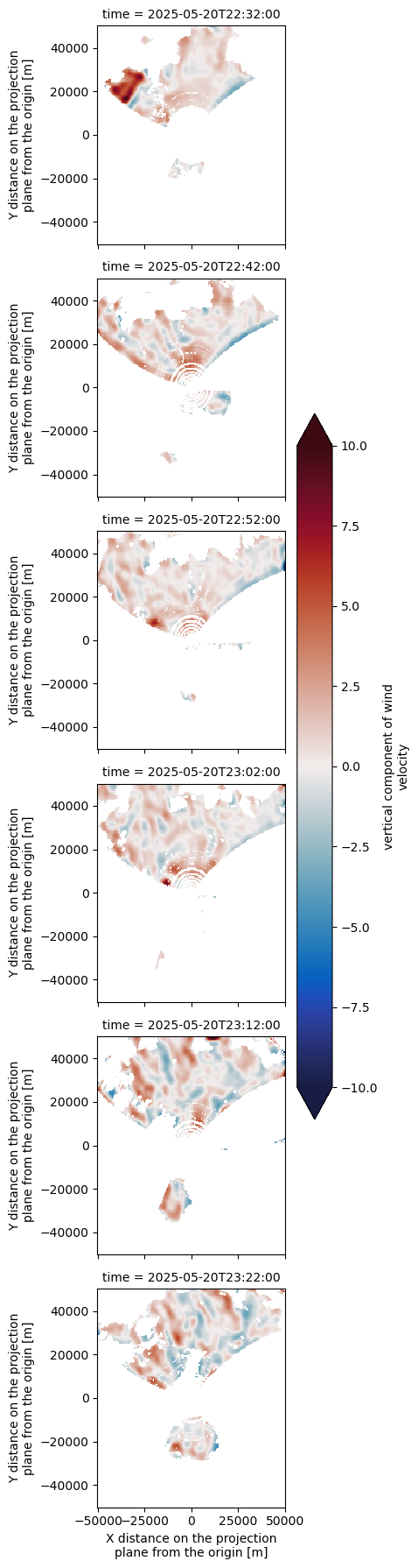
We can take a slice through ~3 km using xarray
ds.sel(z=3000,
       method="nearest",
      ).w.plot(row="time",
               vmin=-10,
               cmap="balance",
       vmax=10)
<xarray.plot.facetgrid.FacetGrid at 0x7f7af09885f0>