First, we’re going to import all the libraries to perform the updraft tracking
import datetime
import shutil
from pathlib import Path
from six.moves import urllib

import numpy as np
import pandas as pd
import xarray as xr

import matplotlib.pyplot as plt
%matplotlib inline

import glob
import cmweather
Now, let’s import tobac:
import tobac
print('using tobac version', str(tobac.__version__))
ERROR 1: PROJ: proj_create_from_database: Open of /opt/conda/share/proj failed
using tobac version 1.6.0
Getting the datasets we’ll be using and opening them, as well as performing initial inspection of the data:
file = sorted(glob.glob("/data/project/ARM_Summer_School_2025/radar/dda/multidop/stonybrook/*")) #Star at the end pulls everything that's in that directory
file
['/data/project/ARM_Summer_School_2025/radar/dda/multidop/stonybrook/armrkhtxconv.20230401.071733.nc',
'/data/project/ARM_Summer_School_2025/radar/dda/multidop/stonybrook/armrkhtxconv.20230401.072813.nc',
'/data/project/ARM_Summer_School_2025/radar/dda/multidop/stonybrook/armrkhtxconv.20230401.074551.nc',
'/data/project/ARM_Summer_School_2025/radar/dda/multidop/stonybrook/armrkhtxconv.20230401.080334.nc',
'/data/project/ARM_Summer_School_2025/radar/dda/multidop/stonybrook/armrkhtxconv.20230401.082641.nc']ds = xr.open_mfdataset(file) #files[0] just for the first file. Add "mf" before "dataset()" to open multiple files
dsLoading...
ds["x"]Loading...
Taking a look at the vertical wind component
ds["vertical_wind_component"].isel(time=0).sel(z=5000).plot(cmap="Spectral_r")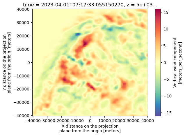
Subsetting data
Given that there are ripples in the w field above ~14 km, we opt to slice our data from 0 to 8 km.
ds = ds.sel(z=slice(0, 8_000))vert_wind = ds["vertical_wind_component"]vert_windLoading...
#vert_wind = vert_wind.drop_vars('z') #This is in case we need to drop the vertical axisSetting up tobac
In this section, we’re going to work with our vertical velocity data without manipulating it. Our goal is to try to understand how to set up tobac.
#Defining the resolution of our data
dxy = 500
dt = 15*60
# Keyword arguments for feature detection step:
parameters_features={}
parameters_features['position_threshold']='weighted_diff'
parameters_features['sigma_threshold']=0.5
parameters_features['min_distance']=0
parameters_features['sigma_threshold']=1
parameters_features['threshold']=[3, 5, 10] #m/s
parameters_features['n_erosion_threshold']=0
parameters_features['n_min_threshold']=3Running tobac for first case
# Perform feature detection and save results:
print('start feature detection based on midlevel column maximum vertical velocity')
Features=tobac.feature_detection_multithreshold(vert_wind,dxy, vertical_cord='z', **parameters_features)
print('feature detection performed start saving features')
#Features.to_hdf(savedir / 'Features.h5', 'table')
print('features saved')start feature detection based on midlevel column maximum vertical velocity
feature detection performed start saving features
features saved
FeaturesLoading...
# Keyword arguments for linking step:
parameters_linking={}
parameters_linking['method_linking']='predict'
parameters_linking['adaptive_stop']=0.5
parameters_linking['adaptive_step']=0.95
parameters_linking['extrapolate']=0
parameters_linking['order']=1
parameters_linking['subnetwork_size']=5
parameters_linking['memory']=0
parameters_linking['time_cell_min']=dt
parameters_linking['method_linking']='predict'
parameters_linking['v_max']=15# Perform linking and save results:
Track=tobac.linking_trackpy(Features,vert_wind,dt=dt,dxy=dxy,**parameters_linking)
#Track.to_hdf(savedir / 'Track.h5', 'table')Frame 4: 37 trajectories present.
TrackLoading...
Track.groupby("cell")["time_cell"].max()cell
-1 NaT
6 0 days 00:10:40.000366449
8 0 days 01:09:08.002762794
9 0 days 00:46:01.007535219
10 0 days 01:09:08.002762794
...
114 0 days 00:23:06.995227575
116 0 days 00:23:06.995227575
117 0 days 00:23:06.995227575
119 0 days 00:23:06.995227575
120 0 days 00:23:06.995227575
Name: time_cell, Length: 65, dtype: timedelta64[ns]Track = Track[Track["cell"] != -1]# Updraft lifetimes of tracked cells:
fig_lifetime,ax_lifetime=plt.subplots()
tobac.plot_lifetime_histogram_bar(Track,axes=ax_lifetime,bin_edges=np.arange(0,120,10),density=False,width_bar=8)
ax_lifetime.set_xlabel('lifetime (min)')
ax_lifetime.set_ylabel('counts')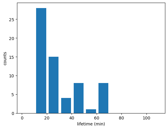
#Segmentation
parameters_segmentation_TWC={}
parameters_segmentation_TWC['method']='watershed'
parameters_segmentation_TWC['threshold']=1 print('Start segmentation based on total water content')
Mask_TWC, Features_TWC = tobac.segmentation_3D(Features, vert_wind, dxy, **parameters_segmentation_TWC)
print('segmentation TWC performed, start saving results to files')
#Mask_TWC.to_netcdf(savedir / 'Mask_Segmentation_TWC.nc', encoding={"segmentation_mask":{"zlib":True, "complevel":4}})
#Features_TWC.to_hdf(savedir / 'Features_TWC.h5','table')
print('segmentation TWC performed and saved')Start segmentation based on total water content
segmentation TWC performed, start saving results to files
segmentation TWC performed and saved
Track[Track["frame"]==0]["x"]5 37940.312830
7 -31421.728172
8 -26278.325532
9 15833.892314
10 -32562.664238
12 -38061.670324
13 -3780.940510
14 -26917.609968
15 -32710.479608
18 31992.417937
19 -7277.339006
21 3756.861052
23 -6125.608090
25 -17317.440601
28 12638.542416
32 4162.764458
36 22530.218180
38 -12989.836650
39 17789.949453
42 25044.362168
44 14926.079326
45 -29107.676279
48 19875.333476
49 37386.993259
50 -27141.171290
52 22373.637336
53 7420.194082
54 26641.250985
56 29257.064484
57 -32650.673805
58 -5729.776139
59 -12347.473716
60 -19576.947832
62 -9287.634917
63 -3091.907193
65 23617.779517
66 -18458.099888
Name: x, dtype: float64ds["vertical_wind_component"].isel(time=0).sel(z=6000).plot(cmap="Spectral_r")
plt.scatter(Track[Track["frame"]==0]["x"], Track[Track["frame"]==0]["y"])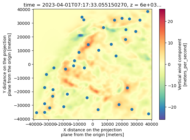
ds["vertical_wind_component"].isel(time=0).max(dim="z").plot(cmap="Spectral_r") #We're going to try to get the wmax. For that, we do .max along the z direction!
plt.scatter(Track[Track["frame"]==0]["x"], Track[Track["frame"]==0]["y"])
Running a new feature detection by taking the maximum w field first
w_wind_max = ds["vertical_wind_component"].max(dim="z")w_wind_maxLoading...
# Keyword arguments for feature detection step:
parameters_features={}
parameters_features['position_threshold']='weighted_diff'
parameters_features['sigma_threshold']=0.5
parameters_features['min_distance']=0
parameters_features['sigma_threshold']=1
parameters_features['threshold']=[3, 5, 10] #m/s
parameters_features['n_erosion_threshold']=0
parameters_features['n_min_threshold']=3# Perform feature detection and save results:
print('start feature detection based on midlevel column maximum vertical velocity')
Features=tobac.feature_detection_multithreshold(w_wind_max,dxy, vertical_cord='z', **parameters_features)
print('feature detection performed start saving features')
print('features saved')start feature detection based on midlevel column maximum vertical velocity
feature detection performed start saving features
features saved
FeaturesLoading...
# Keyword arguments for linking step:
parameters_linking={}
parameters_linking['method_linking']='predict'
parameters_linking['adaptive_stop']=0.5
parameters_linking['adaptive_step']=0.95
parameters_linking['extrapolate']=0
parameters_linking['order']=1
parameters_linking['subnetwork_size']=5
parameters_linking['memory']=0
parameters_linking['time_cell_min']=dt
parameters_linking['method_linking']='predict'
parameters_linking['v_max']=15
# Perform linking and save results:
Track_w_wind_max = tobac.linking_trackpy(Features,w_wind_max,dt=dt,dxy=dxy,**parameters_linking)
#Track.to_hdf(savedir / 'Track.h5', 'table')Frame 4: 37 trajectories present.
Track_w_wind_maxLoading...
Track_w_wind_max.groupby("cell")["time_cell"].max()cell
-1 NaT
2 0 days 01:09:08.002762794
3 0 days 00:28:18.000530958
4 0 days 00:28:18.000530958
8 0 days 01:09:08.002762794
9 0 days 01:09:08.002762794
10 0 days 01:09:08.002762794
11 0 days 00:10:40.000366449
14 0 days 01:09:08.002762794
19 0 days 00:10:40.000366449
22 0 days 00:28:18.000530958
23 0 days 00:28:18.000530958
24 0 days 00:10:40.000366449
29 0 days 01:09:08.002762794
30 0 days 00:28:18.000530958
32 0 days 00:10:40.000366449
33 0 days 00:28:18.000530958
35 0 days 00:10:40.000366449
40 0 days 00:10:40.000366449
42 0 days 01:09:08.002762794
45 0 days 01:09:08.002762794
47 0 days 00:10:40.000366449
48 0 days 00:28:18.000530958
49 0 days 00:46:01.007535219
50 0 days 01:09:08.002762794
52 0 days 01:09:08.002762794
55 0 days 00:10:40.000366449
57 0 days 01:09:08.002762794
58 0 days 00:10:40.000366449
59 0 days 01:09:08.002762794
60 0 days 00:17:38.000164509
61 0 days 00:17:38.000164509
63 0 days 00:35:21.007168770
64 0 days 00:58:28.002396345
67 0 days 00:58:28.002396345
68 0 days 00:58:28.002396345
69 0 days 00:35:21.007168770
70 0 days 00:17:38.000164509
72 0 days 00:40:50.002231836
73 0 days 00:40:50.002231836
74 0 days 00:17:43.007004261
75 0 days 00:40:50.002231836
76 0 days 00:40:50.002231836
77 0 days 00:17:43.007004261
78 0 days 00:40:50.002231836
80 0 days 00:40:50.002231836
81 0 days 00:40:50.002231836
82 0 days 00:40:50.002231836
83 0 days 00:40:50.002231836
94 0 days 00:23:06.995227575
97 0 days 00:23:06.995227575
103 0 days 00:23:06.995227575
104 0 days 00:23:06.995227575
Name: time_cell, dtype: timedelta64[ns]Track_w_wind_max = Track_w_wind_max[Track_w_wind_max["cell"] != -1]# Updraft lifetimes of tracked cells:
fig_lifetime,ax_lifetime=plt.subplots()
tobac.plot_lifetime_histogram_bar(Track_w_wind_max,axes=ax_lifetime,bin_edges=np.arange(0,120,10),density=False,width_bar=8)
ax_lifetime.set_xlabel('lifetime (min)')
ax_lifetime.set_ylabel('counts')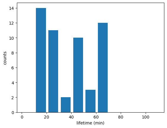
#Segmentation
parameters_segmentation_TWC={}
parameters_segmentation_TWC['method']='watershed'
parameters_segmentation_TWC['threshold']=1
print('Start segmentation based on total water content')
Mask_TWC, Features_TWC = tobac.segmentation_3D(Features, w_wind_max, dxy, **parameters_segmentation_TWC)
print('segmentation TWC performed, start saving results to files')
#Mask_TWC.to_netcdf(savedir / 'Mask_Segmentation_TWC.nc', encoding={"segmentation_mask":{"zlib":True, "complevel":4}})
#Features_TWC.to_hdf(savedir / 'Features_TWC.h5','table')
print('segmentation TWC performed and saved')Start segmentation based on total water content
segmentation TWC performed, start saving results to files
segmentation TWC performed and saved
Track_w_wind_max[Track_w_wind_max["frame"]==0]["x"]
1     29599.634976
2    -38888.974631
3      3887.210415
7    -17266.658546
8    -36712.569711
9    -32816.936701
10    32244.689285
13   -26352.315936
18     4227.495128
21    28293.928498
22    -6937.500092
23      181.802757
28    33766.555632
29   -29544.800736
31    17798.734025
32   -19532.618183
34    33244.641395
39    22295.156665
41    22548.944155
44     7863.344224
46    15078.502408
47    32452.991398
48    19960.347453
49    28223.303629
51    37140.800796
54    23564.548715
56   -10336.796840
57   -18269.711623
58    -3292.726903
Name: x, dtype: float64
ds["vertical_wind_component"].isel(time=0).max(dim="z").plot(cmap="Spectral_r") #We're going to try to get the wmax. For that, we do .max along the z direction!
plt.scatter(Track_w_wind_max[Track_w_wind_max["frame"]==0]["x"], Track_w_wind_max[Track_w_wind_max["frame"]==0]["y"])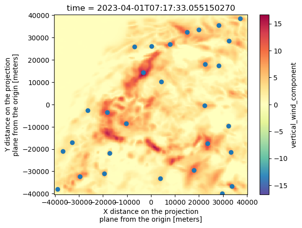
w_wind_max.isel(time=0).plot()
plt.scatter(Track_w_wind_max[Track_w_wind_max["frame"]==0]["x"], Track_w_wind_max[Track_w_wind_max["frame"]==0]["y"])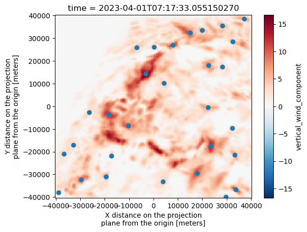
w_wind_max.isel(time=1).plot()
plt.scatter(Track_w_wind_max[Track_w_wind_max["frame"]==1]["x"], Track_w_wind_max[Track_w_wind_max["frame"]==1]["y"])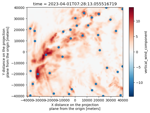
Working on animating the detected features
Animation for w_max_tracking
#Setting up a for loop to plot more figures
w_wind_max.isel(time=2).plot()
plt.scatter(Track_w_wind_max[Track_w_wind_max["frame"]==2]["x"], Track_w_wind_max[Track_w_wind_max["frame"]==2]["y"])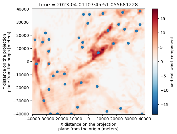
single_time = Track_w_wind_max.time.unique()[2]
single_time
Timestamp('2023-04-01 07:45:51.055681228')Track_w_wind_max.loc[(Track_w_wind_max.time == single_time) & (Track_w_wind_max.threshold_value == 10)]Loading...
def subset_column(ds, time, x, y):
    return ds.sel(time=time, x=x, y=y, method='nearest')
single_cell = Track_w_wind_max.loc[Track_w_wind_max.cell == 42]
ds_list = []
for time in single_cell.time.values:
row = single_cell.loc[single_cell.time == time]
ds_list.append(subset_column(ds, time=row.time.values, x=row.x.values, y=row.y.values))
single_cell_ds = xr.concat(ds_list, dim='time')
single_cell_ds
single_cell_ds.vertical_wind_component.max(["y", "x"]).plot(y='z')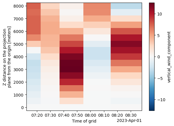
# Filter for a single cell (cell 42)
single_cell = Track_w_wind_max.loc[Track_w_wind_max.cell == 42]
# Subset data at each time step using x, y, and time
ds_list = []
for time in single_cell.time.values:
row = single_cell.loc[single_cell.time == time]
ds_list.append(subset_column(ds, time=row.time.values, x=row.x.values, y=row.y.values))
# Concatenate all time slices into a single dataset
single_cell_ds = xr.concat(ds_list, dim='time')
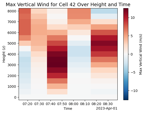
# Plot the max vertical wind component over time and height
plot = single_cell_ds.vertical_wind_component.max(["y", "x"]).plot(
y='z',
cbar_kwargs={'label': 'Max Vertical Wind (m/s)'} # custom colorbar label
)
# Add a custom title and axis labels
plt.title("Max Vertical Wind for Cell 42 Over Height and Time", fontsize=14)
plt.xlabel("Time")
plt.ylabel("Height (z)")
# Show plot
plt.show()
ax = plt.subplot(111)
#ds.sel(z=5000).isel(time=2).vertical_wind_component.plot()
ds.sel(z=3000).isel(time=2).radar_network_reflectivity.plot(cmap="Spectral_r", vmin=-20, vmax=70)
Track_w_wind_max.loc[Track_w_wind_max.cell == 42].plot.scatter(x="x", y='y', ax=ax, c="threshold_value", cmap="Reds")
<Axes: title={'center': 'time = 2023-04-01T07:45:51.055681228, z = 3e+03...'}, xlabel='x', ylabel='y'>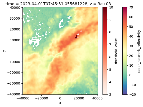
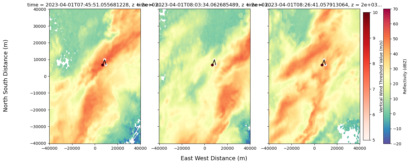
Track_w_wind_max.loc[Track_w_wind_max.cell == 83]Loading...
y_line = Track_w_wind_max.groupby('cell')['y'].apply(list).loc[83]y_line[6651.333210487742, 9803.516653223049, 6774.890043359406]x_line = Track_w_wind_max.groupby('cell')['x'].apply(list).loc[83]#ax = plt.subplot(111)
#ds.sel(z=5000).isel(time=2).vertical_wind_component.plot()
#Track_w_wind_max.loc[Track_w_wind_max.cell == 83].plot.scatter(x="x", y='y', ax=ax, c="threshold_value", cmap="Reds")
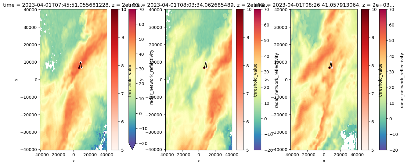
fig, axs = plt.subplots(1, 3, figsize=(15, 6))
y1 = ds.sel(z=2000).isel(time=2).radar_network_reflectivity.plot(cmap="Spectral_r", vmin=-20, vmax=70, ax = axs[0])
y2 = ds.sel(z=2000).isel(time=3).radar_network_reflectivity.plot(cmap="Spectral_r", vmin=-20, vmax=70, ax = axs[1])
y3 = ds.sel(z=2000).isel(time=4).radar_network_reflectivity.plot(cmap="Spectral_r", vmin=-20, vmax=70, ax = axs[2])
scatter_data = Track_w_wind_max.loc[Track_w_wind_max.cell == 83]
#axs[0].plot(x_line, y_line)
#axs[1].plot(x_line, y_line)
#axs[2].plot(x_line, y_line)
# Add the scatter and line plot to each subplot
for ax in axs:
scatter_data.plot.scatter(x="x", y="y", ax=ax, c="threshold_value", cmap="Reds")
ax.plot(x_line, y_line, color='black') # Optional: specify color or linestyle
fig, axs = plt.subplots(1, 3, figsize=(15, 6), sharex=True, sharey=True)

# Plotting (as before)
mappable_refl = ds.sel(z=2000).isel(time=2).radar_network_reflectivity.plot(
    cmap="Spectral_r", vmin=-20, vmax=70, ax=axs[0], add_colorbar=False)
ds.sel(z=2000).isel(time=3).radar_network_reflectivity.plot(
    cmap="Spectral_r", vmin=-20, vmax=70, ax=axs[1], add_colorbar=False)
ds.sel(z=2000).isel(time=4).radar_network_reflectivity.plot(
    cmap="Spectral_r", vmin=-20, vmax=70, ax=axs[2], add_colorbar=False)

# Scatter and lines
scatter_data = Track_w_wind_max.loc[Track_w_wind_max.cell == 83]
sc = axs[0].scatter(scatter_data["x"], scatter_data["y"], c=scatter_data["threshold_value"], cmap="Reds")
for ax in axs:
    ax.scatter(scatter_data["x"], scatter_data["y"], c=scatter_data["threshold_value"], cmap="Reds")
    ax.plot(x_line, y_line, color='black')
    ax.set_xlabel('')  # Remove individual x labels
    ax.set_ylabel('')  # Remove individual y labels

# Shared axis labels
fig.supxlabel("East West Distance (m)", fontsize=14)
fig.supylabel("North South Distance (m)", fontsize=14)

# Shared colorbars
cbar1 = fig.colorbar(mappable_refl, ax=axs, orientation='vertical', fraction=0.02, pad=0.04)
cbar1.set_label('Reflectivity (dBZ)')
cbar2 = fig.colorbar(sc, ax=axs, orientation='vertical', fraction=0.02, pad=0.01)
cbar2.set_label('Vertical Wind Threshold Value (m/s)')
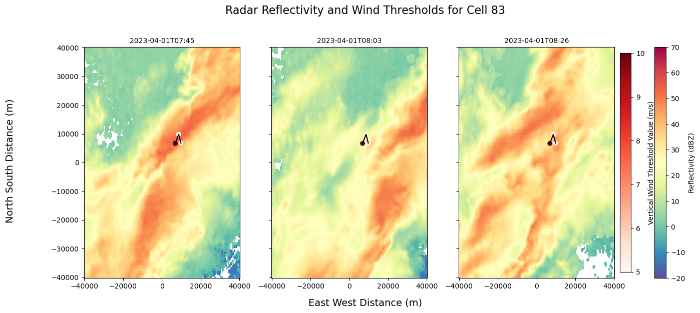
fig, axs = plt.subplots(1, 3, figsize=(15, 6), sharex=True, sharey=True)
fig.suptitle("Radar Reflectivity and Wind Thresholds for Cell 83", fontsize=16, y=1.02)

# Reflectivity plots without auto-labels
mappable_refl = ds.sel(z=2000).isel(time=2).radar_network_reflectivity.plot(
    cmap="Spectral_r", vmin=-20, vmax=70, ax=axs[0], add_colorbar=False, add_labels=False)
ds.sel(z=2000).isel(time=3).radar_network_reflectivity.plot(
    cmap="Spectral_r", vmin=-20, vmax=70, ax=axs[1], add_colorbar=False, add_labels=False)
ds.sel(z=2000).isel(time=4).radar_network_reflectivity.plot(
    cmap="Spectral_r", vmin=-20, vmax=70, ax=axs[2], add_colorbar=False, add_labels=False)

# Custom titles (example using time values)
axs[0].set_title(str(ds.time.values[2])[:16], fontsize=10)
axs[1].set_title(str(ds.time.values[3])[:16], fontsize=10)
axs[2].set_title(str(ds.time.values[4])[:16], fontsize=10)

# Scatter and lines
scatter_data = Track_w_wind_max.loc[Track_w_wind_max.cell == 83]
sc = axs[0].scatter(scatter_data["x"], scatter_data["y"], c=scatter_data["threshold_value"], cmap="Reds")
for ax in axs:
    ax.scatter(scatter_data["x"], scatter_data["y"], c=scatter_data["threshold_value"], cmap="Reds")
    ax.plot(x_line, y_line, color='black')
    ax.set_xlabel('')
    ax.set_ylabel('')

# Shared axis labels
fig.supxlabel("East West Distance (m)", fontsize=14)
fig.supylabel("North South Distance (m)", fontsize=14)

# Shared colorbars
cbar1 = fig.colorbar(mappable_refl, ax=axs, orientation='vertical', fraction=0.02, pad=0.04)
cbar1.set_label('Reflectivity (dBZ)')

cbar2 = fig.colorbar(sc, ax=axs, orientation='vertical', fraction=0.02, pad=0.01)
cbar2.set_label('Vertical Wind Threshold Value (m/s)')

plt.savefig('cell_83_graph.pdf', dpi=300)
plt.savefig("cell_83_graph.png", dpi=300, bbox_inches='tight')
single_cell = Track_w_wind_max.loc[Track_w_wind_max.cell == 83]
ds_list = []
for time in single_cell.time.values:
    row = single_cell.loc[single_cell.time == time]
    ds_list.append(subset_column(ds, time=row.time.values, x=row.x.values, y=row.y.values))

single_cell_ds = xr.concat(ds_list, dim='time')
single_cell_ds
single_cell_ds.vertical_wind_component.max(["y", "x"]).plot(y='z')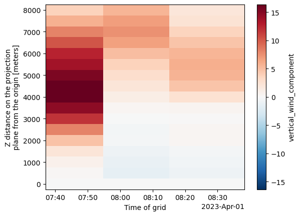
# Filter for cell 83
single_cell = Track_w_wind_max.loc[Track_w_wind_max.cell == 83]

# Subset data at each time step
ds_list = []
for time in single_cell.time.values:
    row = single_cell.loc[single_cell.time == time]
    ds_list.append(subset_column(ds, time=row.time.values, x=row.x.values, y=row.y.values))

# Concatenate all time slices
single_cell_ds = xr.concat(ds_list, dim='time')

# Plot max vertical wind component with custom colorbar label
plot = single_cell_ds.vertical_wind_component.max(["y", "x"]).plot(
    y='z',
    cbar_kwargs={'label': 'Max Vertical Wind (m/s)'}
)

# Add figure title and axes labels
plt.title("Max Vertical Wind for Cell 83 Over Height and Time", fontsize=14)
plt.xlabel("Time")
plt.ylabel("Height (z)")

# Show plot

plt.savefig("cell_83_secondgraph.png", dpi=300)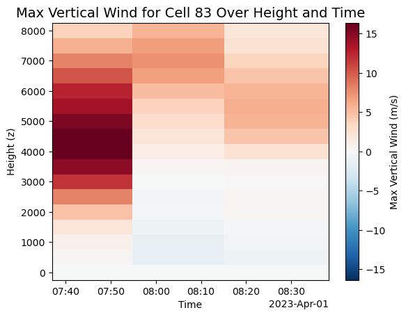
<Figure size 640x480 with 0 Axes>single_cell_ds.vertical_wind_component.max(dim=["x", "y", "z"]).plot()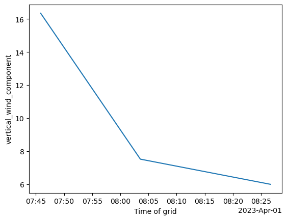
Running some other tests
ax = plt.subplot(111)
#ds.sel(z=5000).isel(time=2).vertical_wind_component.plot()
ds.sel(z=2000).isel(time=2).radar_network_reflectivity.plot(cmap="Spectral_r", vmin=-20, vmax=70)
Track_w_wind_max.loc[Track_w_wind_max.cell == 83].plot. scatter(x="x", y='y', ax=ax, c="threshold_value", cmap="Reds")
<Axes: title={'center': 'time = 2023-04-01T07:45:51.055681228, z = 2e+03...'}, xlabel='x', ylabel='y'>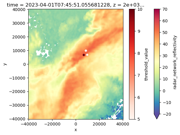
Track_w_wind_max.loc[Track_w_wind_max.cell == 42]Loading...
y_line2 = Track_w_wind_max.groupby('cell')['y'].apply(list).loc[42]
x_line2 = Track_w_wind_max.groupby('cell')['x'].apply(list).loc[42]
fig, axs = plt.subplots(1, 5, figsize=(15, 6), sharex=True, sharey=True)
# Plotting (as before)
mappable_refl = ds.sel(z=2000).isel(time=0).radar_network_reflectivity.plot(
cmap="Spectral_r", vmin=-20, vmax=70, ax=axs[0], add_colorbar=False)
ds.sel(z=2000).isel(time=1).radar_network_reflectivity.plot(
cmap="Spectral_r", vmin=-20, vmax=70, ax=axs[1], add_colorbar=False)
ds.sel(z=2000).isel(time=2).radar_network_reflectivity.plot(
cmap="Spectral_r", vmin=-20, vmax=70, ax=axs[2], add_colorbar=False)
ds.sel(z=2000).isel(time=3).radar_network_reflectivity.plot(
cmap="Spectral_r", vmin=-20, vmax=70, ax=axs[3], add_colorbar=False)
ds.sel(z=2000).isel(time=4).radar_network_reflectivity.plot(
cmap="Spectral_r", vmin=-20, vmax=70, ax=axs[4], add_colorbar=False)
# Scatter and lines
scatter_data = Track_w_wind_max.loc[Track_w_wind_max.cell == 42]
sc = axs[0].scatter(scatter_data["x"], scatter_data["y"], c=scatter_data["threshold_value"], cmap="Reds")
for ax in axs:
ax.scatter(scatter_data["x"], scatter_data["y"], c=scatter_data["threshold_value"], cmap="Reds")
ax.plot(x_line2, y_line2, color='black')
ax.set_xlabel('') # Remove individual x labels
ax.set_ylabel('') # Remove individual y labels
# Shared axis labels
fig.supxlabel("East West Distance (m)", fontsize=14)
fig.supylabel("North South Distance (m)", fontsize=14)
# Shared colorbars
cbar1 = fig.colorbar(mappable_refl, ax=axs, orientation='vertical', fraction=0.02, pad=0.04)
cbar1.set_label('Reflectivity (dBZ)')
cbar2 = fig.colorbar(sc, ax=axs, orientation='vertical', fraction=0.02, pad=0.01)
cbar2.set_label('Vertical Wind Threshold Value (m/s)')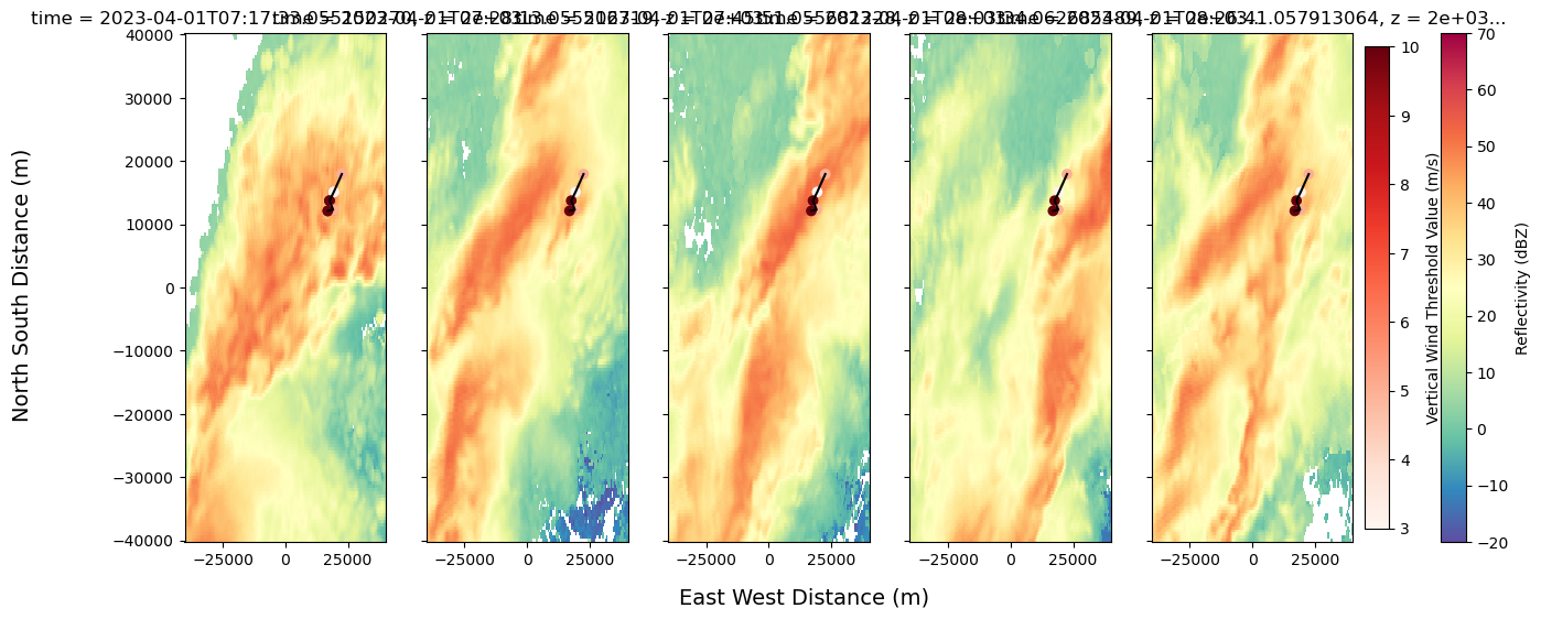
fig, axs = plt.subplots(1, 5, figsize=(15, 6), sharex=True, sharey=True)
fig.suptitle("Radar Reflectivity and Wind Thresholds for Cell 42", fontsize=16, y=1.02)

# Reflectivity plots with suppressed auto-labels
mappable_refl = ds.sel(z=2000).isel(time=0).radar_network_reflectivity.plot(
    cmap="Spectral_r", vmin=-20, vmax=70, ax=axs[0], add_colorbar=False, add_labels=False)
ds.sel(z=2000).isel(time=1).radar_network_reflectivity.plot(
    cmap="Spectral_r", vmin=-20, vmax=70, ax=axs[1], add_colorbar=False, add_labels=False)
ds.sel(z=2000).isel(time=2).radar_network_reflectivity.plot(
    cmap="Spectral_r", vmin=-20, vmax=70, ax=axs[2], add_colorbar=False, add_labels=False)
ds.sel(z=2000).isel(time=3).radar_network_reflectivity.plot(
    cmap="Spectral_r", vmin=-20, vmax=70, ax=axs[3], add_colorbar=False, add_labels=False)
ds.sel(z=2000).isel(time=4).radar_network_reflectivity.plot(
    cmap="Spectral_r", vmin=-20, vmax=70, ax=axs[4], add_colorbar=False, add_labels=False)

# Add smaller custom titles using time values
for i in range(5):
    time_str = str(ds.time.values[i])[:16]  # Shorten for readability
    axs[i].set_title(f"Time: {time_str}", fontsize=10)

# Scatter and lines
scatter_data = Track_w_wind_max.loc[Track_w_wind_max.cell == 42]
sc = axs[0].scatter(scatter_data["x"], scatter_data["y"], c=scatter_data["threshold_value"], cmap="Reds")
for ax in axs:
    ax.scatter(scatter_data["x"], scatter_data["y"], c=scatter_data["threshold_value"], cmap="Reds")
    ax.plot(x_line2, y_line2, color='black')
    ax.set_xlabel('')
    ax.set_ylabel('')

# Shared axis labels
fig.supxlabel("East West Distance (m)", fontsize=14)
fig.supylabel("North South Distance (m)", fontsize=14)

# Shared colorbars
cbar1 = fig.colorbar(mappable_refl, ax=axs, orientation='vertical', fraction=0.02, pad=0.04)
cbar1.set_label('Reflectivity (dBZ)')

cbar2 = fig.colorbar(sc, ax=axs, orientation='vertical', fraction=0.02, pad=0.01)
cbar2.set_label('Vertical Wind Threshold Value (m/s)')
plt.savefig("cell_42_graph.png", dpi=300, bbox_inches='tight')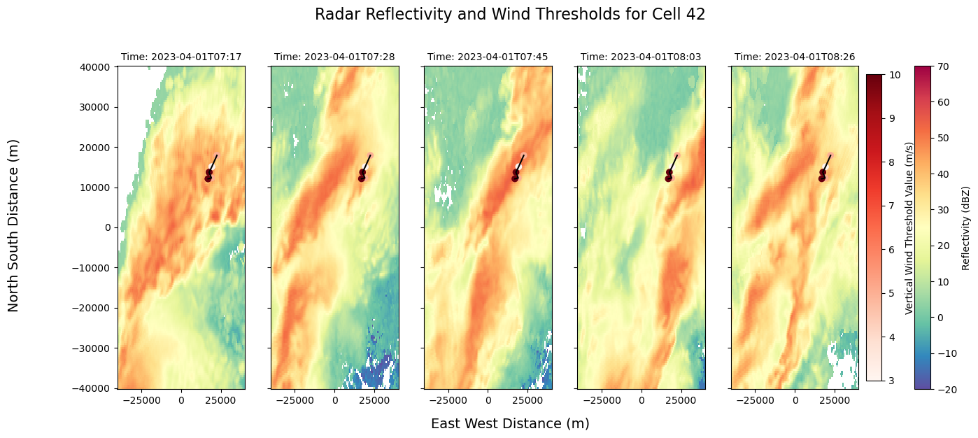
x_line2[22548.94415473999,
19353.739649537958,
17639.602952613473,
19085.857258161184,
16971.86614109041]y_line2[17931.799437239868,
15105.755774743593,
13729.23953881,
12295.767178448572,
12112.628000649096]